ELIXIR Spatial course
Spatial & single-cell data integration
Day 2 - Practical 5
7th October 2026
Benedetta Manzato (LUMC) & Emma Vonk (LUMC)
- Dataset description
- Spatial imputation with SpaGE and Tangram
- Cell deconvolution with Cell2location
import os
import warnings
import anndata as ad
import matplotlib.pyplot as plt
import numpy as np
import pandas as pd
import scanpy as sc
warnings.filterwarnings("ignore")
# Display the version of important packages for reproducibility
sc.logging.print_header()
# Set the default aesthetics for Scanpy plots
sc.set_figure_params(facecolor='white', figsize=(8, 8)) # White background, figure size 8x8
sc.settings.verbosity = 0 # Set verbosity to show only errors (0) # errors (0), warnings (1), info (2), hints (3)
We create an output folder in your local space to save outputs:
folder_path = './outputs/'
if not os.path.exists(folder_path):
os.makedirs(folder_path)
print(f"Folder created: {folder_path}")
else:
print(f"Folder already exists: {folder_path}")
Folder created: ./outputs/
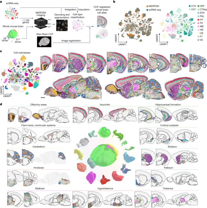
Dataset: MERFISH Spatial Transcriptomics of Adult Mouse Brain (Zhuang‑ABCA‑1)
We will use the Zhuang-ABCA-1 dataset: 4.2 million cell spatial transcriptomics dataset spanning 147 coronal sections with a 1122 gene panel. 2.8 million cells passed cell classification confidence score threshold and displayed in the ABC atlas.
We decided to work with one section only, the one that captures most cells (section 80).
Read data
We will read the AnnData object that has been filtered to have only section 80 and QC was performed from the authors of the study. The data can be found in the Zenodo directory provided.
adata_section = ad.read_h5ad("../data/Practical5/adata_section80.h5ad")
The dataset was obtain with a targeted / imaging-based technology and not the whole transcriptome is measured, just a limited gene panel.
- Question: how many genes are measured?
Reminder from Practical 0: Spatial coordinates, being metadata about cells/spots are stored either in .obs or .obsm Spot metadata also contains info about class, subclass, neurotransmitter, patient metadata and section.
adata_section.obs.head()
| brain_section_label | feature_matrix_label | donor_label | donor_genotype | donor_sex | cluster_alias | x | y | z | subclass_confidence_score | ... | neurotransmitter | class | subclass | supertype | cluster | neurotransmitter_color | class_color | subclass_color | supertype_color | cluster_color | |
|---|---|---|---|---|---|---|---|---|---|---|---|---|---|---|---|---|---|---|---|---|---|
| cell_label | |||||||||||||||||||||
| 299794030110334465835331169565547130392 | Zhuang-ABCA-1.080 | Zhuang-ABCA-1 | Zhuang-ABCA-1 | wt/wt | F | 196 | 5.873824 | 1.246374 | 6.757411 | 0.951445 | ... | Glut | 01 IT-ET Glut | 006 L4/5 IT CTX Glut | 0027 L4/5 IT CTX Glut_5 | 0097 L4/5 IT CTX Glut_5 | #2B93DF | #FA0087 | #3DCCB7 | #639917 | #1C0099 |
| 66045375924099067525605874805924532486 | Zhuang-ABCA-1.080 | Zhuang-ABCA-1 | Zhuang-ABCA-1 | wt/wt | F | 196 | 5.066814 | 1.215444 | 6.757411 | 0.990889 | ... | Glut | 01 IT-ET Glut | 006 L4/5 IT CTX Glut | 0027 L4/5 IT CTX Glut_5 | 0097 L4/5 IT CTX Glut_5 | #2B93DF | #FA0087 | #3DCCB7 | #639917 | #1C0099 |
| 116791314340621211157298988846240231316 | Zhuang-ABCA-1.080 | Zhuang-ABCA-1 | Zhuang-ABCA-1 | wt/wt | F | 196 | 4.681061 | 1.287158 | 6.757411 | 0.972796 | ... | Glut | 01 IT-ET Glut | 006 L4/5 IT CTX Glut | 0027 L4/5 IT CTX Glut_5 | 0097 L4/5 IT CTX Glut_5 | #2B93DF | #FA0087 | #3DCCB7 | #639917 | #1C0099 |
| 13950435409550353848526753205083905255 | Zhuang-ABCA-1.080 | Zhuang-ABCA-1 | Zhuang-ABCA-1 | wt/wt | F | 174 | 4.708601 | 1.292049 | 6.757411 | 0.995666 | ... | Glut | 01 IT-ET Glut | 006 L4/5 IT CTX Glut | 0023 L4/5 IT CTX Glut_1 | 0069 L4/5 IT CTX Glut_1 | #2B93DF | #FA0087 | #3DCCB7 | #3B9900 | #997145 |
| 147436316185400258367147717470263928395 | Zhuang-ABCA-1.080 | Zhuang-ABCA-1 | Zhuang-ABCA-1 | wt/wt | F | 174 | 4.729919 | 1.285492 | 6.757411 | 0.999973 | ... | Glut | 01 IT-ET Glut | 006 L4/5 IT CTX Glut | 0023 L4/5 IT CTX Glut_1 | 0069 L4/5 IT CTX Glut_1 | #2B93DF | #FA0087 | #3DCCB7 | #3B9900 | #997145 |
5 rows × 22 columns
Some spatial tools require the spatial coordinates can be stored as spatial or X_spatial
# Add X_spatial to the right field
x_spatial = np.array(adata_section.obs[['x','y']])
adata_section.obsm['X_spatial'] = x_spatial
adata_section.obsm['X_spatial']
array([[5.87382373, 1.24637434],
[5.0668137 , 1.21544436],
[4.68106119, 1.28715849],
...,
[0.97304079, 4.80513099],
[0.86566165, 4.29416095],
[0.84111779, 3.8952338 ]], shape=(37068, 2))
import gc
# collect garbage
gc.collect()
35
Prediction of spatial patterns for unmeasured genes using scRNA-seq data with SpaGE
SpaGE: Spatial Gene Enhancement using scRNA-seq (Abdelaal et al. 2020)
SpaGE cannot be installed using pip or conda, so we have to clone the Git repository.
![ -d SpaGE ] || (wget -qO- https://github.com/tabdelaal/SpaGE/archive/refs/heads/master.tar.gz | tar xz && mv SpaGE-master SpaGE)
Now that the sourced vode of SpaGE is cloned to our folder, lets append the path.
import sys
sys.path.append("SpaGE")
from SpaGE.main import SpaGE
SpaGE is now all set up! Lets continue with the rest of the analysis.
import scipy.stats as st

SpaGE takes as input the (targeted) spatial dataset (query) and a single-cell RNA dataset used as reference. The two datasets should be generated under the same conditions (same species, tissue, region) as much as possible.
We will use Mouse whole-brain transcriptomic cell type atlas (Hongkui Zeng).This scRNAseq dataset profiled 7 million cells (approximately 4.0 million cells passing quality control). More in detail:
1.7 million single cell transcriptomes spanning the whole adult mouse brain using 10Xv2 chemistry (WMB-10Xv2)
2.3 million single cell transcriptomes spanning the whole adult mouse brain using 10Xv3 chemistry (WMB-10Xv3)
1687 single cell transcriptomes spanning the whole adult mouse brain using the 10X Multiome chemistry (WMB-10XMulti)
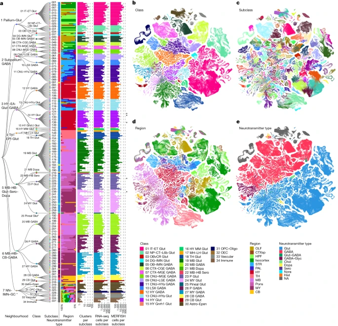
The size is of the combined single-cell object from AbcProjectCache is around 280GB. For this reason, the three objects have been previously downloaded, concatenated, preprocessed and subsetted to obtain 28981 cells. For your knowledge, you can find all the steps in obtain_scref.py.
Let's read the resulting single-cell AnnData object:
adata_sc = ad.read_h5ad("../data/Practical5/sc_adata_1percent.h5ad")
Inspect the object:
adata_sc
AnnData object with n_obs × n_vars = 28981 × 32285
obs: 'cell_barcode', 'barcoded_cell_sample_label', 'library_label', 'feature_matrix_label', 'entity', 'brain_section_label', 'library_method', 'region_of_interest_acronym', 'donor_label', 'donor_genotype', 'donor_sex', 'dataset_label', 'x', 'y', 'cluster_alias'
layers: None (.X)
adata_sc.obs.head()
| cell_barcode | barcoded_cell_sample_label | library_label | feature_matrix_label | entity | brain_section_label | library_method | region_of_interest_acronym | donor_label | donor_genotype | donor_sex | dataset_label | x | y | cluster_alias | |
|---|---|---|---|---|---|---|---|---|---|---|---|---|---|---|---|
| cell_label | |||||||||||||||
| GTATTCTCAGCTATTG-045_C01 | GTATTCTCAGCTATTG | 045_C01 | L8TX_180829_01_C10 | WMB-10Xv2-TH | cell | NaN | 10Xv2 | TH | Snap25-IRES2-Cre;Ai14-407905 | Snap25-IRES2-Cre/wt;Ai14(RCL-tdT)/wt | F | WMB-10Xv2 | 12.420248 | -10.367616 | 5076 |
| GTGTGATCACCAGCGT-468_A02 | GTGTGATCACCAGCGT | 468_A02 | L8TX_201217_01_D07 | WMB-10Xv3-MB | cell | NaN | 10Xv3 | MB | Snap25-IRES2-Cre;Ai14-556231 | Ai14(RCL-tdT)/wt | F | WMB-10Xv3 | 1.571478 | 23.592803 | 14956 |
| TAACCAGCACCAAATC-204.2_A01 | TAACCAGCACCAAATC | 204.2_A01 | L8TX_200122_01_F12 | WMB-10Xv3-MB | cell | NaN | 10Xv3 | MB | Snap25-IRES2-Cre;Ai14-504535 | Snap25-IRES2-Cre/wt;Ai14(RCL-tdT)/wt | F | WMB-10Xv3 | -12.491472 | 11.322906 | 5231 |
| AGCGTCGGTTCAGCGC-420_C06 | AGCGTCGGTTCAGCGC | 420_C06 | L8TX_201106_01_G03 | WMB-10Xv3-MB | cell | NaN | 10Xv3 | MB | Snap25-IRES2-Cre;Ai14-551017 | Ai14(RCL-tdT)/wt | M | WMB-10Xv3 | -10.406498 | 11.711900 | 5230 |
| AGACAAAAGAACTCCT-278_B03 | AGACAAAAGAACTCCT | 278_B03 | L8TX_200702_01_H01 | WMB-10Xv3-TH | cell | NaN | 10Xv3 | TH | Snap25-IRES2-Cre;Ai14-529474 | Snap25-IRES2-Cre/wt;Ai14(RCL-tdT)/wt | F | WMB-10Xv3 | 5.455338 | -13.476950 | 5101 |
In this case the feature metadata are stored in a separate csv. We need to read read and then add them to the right field in the AnnData object
- Add feature metadata to the AnnData object
We previously made sure that the genes in the csv file are sorted in the same way as the ones already present in the AnnData object, so you will just need to add it to the right field now)
# read
genes = pd.read_csv("../data/Practical5/gene.csv",index_col=0)
genes.head()
| gene_symbol | name | mapped_ncbi_identifier | comment | |
|---|---|---|---|---|
| gene_identifier | ||||
| ENSMUSG00000051951 | Xkr4 | X-linked Kx blood group related 4 | NCBIGene:497097 | NaN |
| ENSMUSG00000089699 | Gm1992 | predicted gene 1992 | NaN | NaN |
| ENSMUSG00000102331 | Gm19938 | predicted gene, 19938 | NaN | NaN |
| ENSMUSG00000102343 | Gm37381 | predicted gene, 37381 | NaN | NaN |
| ENSMUSG00000025900 | Rp1 | retinitis pigmentosa 1 (human) | NCBIGene:19888 | NaN |
# add
adata_sc.var = genes
# Reset the index to turn the current index into a column
adata_sc.var.reset_index(inplace=True)
adata_sc.var.set_index('gene_symbol', inplace=True)
adata_sc.var.head()
| gene_identifier | name | mapped_ncbi_identifier | comment | |
|---|---|---|---|---|
| gene_symbol | ||||
| Xkr4 | ENSMUSG00000051951 | X-linked Kx blood group related 4 | NCBIGene:497097 | NaN |
| Gm1992 | ENSMUSG00000089699 | predicted gene 1992 | NaN | NaN |
| Gm19938 | ENSMUSG00000102331 | predicted gene, 19938 | NaN | NaN |
| Gm37381 | ENSMUSG00000102343 | predicted gene, 37381 | NaN | NaN |
| Rp1 | ENSMUSG00000025900 | retinitis pigmentosa 1 (human) | NCBIGene:19888 | NaN |
# collect garbage
gc.collect()
13
Do some pre-processing for SpaGE:
# 1) Filter cells with < 10 expressed genes (counts > 0)
# Scanpy expects "min_genes" to count number of genes per cell (non-zero entries)
sc.pp.filter_cells(adata_sc, min_genes=20) # modifies adata_sc in-place
print(f"After sc.pp.filter_cells: {adata_sc.n_obs} cells, {adata_sc.n_vars} genes")
# 2) Per-cell normalization to counts-per-million (CPM) and log1p
# normalize_total works row-wise (per observation). target_sum=1e6 replicates your earlier scale.
sc.pp.normalize_total(adata_sc, target_sum=1e6, inplace=True) # scales rows so row-sum == 1e6
sc.pp.log1p(adata_sc) # in-place log(1 + X). Works with sparse X.
print("Applied per-cell normalize_total(target_sum=1e6) + log1p.")
# Optional step: memory efficiency purpose only!
# Compute HVGs using Seurat v3 flavor. This writes adata_sc.var['highly_variable'].
# You can change flavor to 'cell_ranger' or 'seurat_v3' depending on preference.
sc.pp.highly_variable_genes(adata_sc, n_top_genes=10000, flavor='seurat_v3', subset=False, inplace=True)
# Subset to keep only HVGs (creates a smaller AnnData)
hv_mask = adata_sc.var['highly_variable'].values.astype(bool)
print(f"Found {hv_mask.sum()} HVGs (requested {10000}). Subsetting AnnData...")
adata_sc = adata_sc[:, hv_mask].copy()
After sc.pp.filter_cells: 28981 cells, 32285 genes
Applied per-cell normalize_total(target_sum=1e6) + log1p.
Found 10007 HVGs (requested 10000). Subsetting AnnData...
- How many genes do the spatial and single-cell data set have in common?
- How many genes are measured in the single-cell dataset that are not measured in the spatial dataset?
## use .intersection
gene_intersection = set(adata_sc.var_names) & set(adata_section.var_names)
## use a set operation
genes_not_intersection = set(adata_sc.var_names) - set(adata_section.var_names)
print(f"Number of genes measured both in the sc and spatial datasets: {len(gene_intersection)}")
print(f"Number of genes measured in the sc reference only (after HVG): {len(genes_not_intersection)}")
Number of genes measured both in the sc and spatial datasets: 881 Number of genes measured in the sc reference only (after HVG): 9114
sc.pp.normalize_total(adata_section, target_sum=1_000_000, inplace=True)
sc.pp.log1p(adata_section)
Let's find some brain-specific genes to predict with SpaGE
brain_region_specific_genes = [
"Bcl11b", "Cux2", "Fezf2", "Tbr1", "Satb2", # isocortex
"Foxp2", # Striatum specific
"Penk", # Basal ganglia specific
"Zic1", # Cerebellum specific
"Hoxb2", # Hindbrain specific
"Dlx6", # Subpallium specific
]
Let's split them in overlap_genes (measured in spatial dataset and sc reference) and non_overlap_genes (unmeasured in the spatial dataset)
# Checking for genes from brain_region_specific_genes that are measured by spatial data
overlap_genes = list(set(adata_section.var.index) & set(brain_region_specific_genes))
overlap_genes
['Bcl11b', 'Zic1', 'Satb2', 'Fezf2', 'Cux2', 'Dlx6', 'Penk']
# Checking for genes from brain_region_specific_genes that are NOT measured by spatial data
non_overlap_genes = list(set(brain_region_specific_genes) - set(overlap_genes))
non_overlap_genes
['Tbr1', 'Hoxb2', 'Foxp2']
Leave-one-gene-out cross validation
Since ground-truth is available, we can leave out the measured (spatial) genes, predict their expression with SpaGE and then compare it to the real expression.
# sc df
RNA_data = adata_sc.to_df()
RNA_data = RNA_data.T
# spatial
spatial_data = adata_section.to_df()
Define the function to predict genes measured in the spatial dataset to have a ground truth and plot the measured expression next to the predicted one.
def predicted_GE_LOOCV(Gene_set, spatial_data, RNA_data):
# Initialize an empty DataFrame to store the predicted values
predicted_df = pd.DataFrame(index=spatial_data.index)
for i in Gene_set:
# Predict the expression of the current gene using the SpaGE method
Imp_Genes = SpaGE(spatial_data.drop(i, axis=1), RNA_data.T, n_pv=30, genes_to_predict=[i])
Imp_Genes.index = spatial_data.index
# Add the predicted values for the current gene as a new column in the DataFrame
predicted_df[i] = Imp_Genes[i]
return predicted_df
predicted_df_loocv = pd.read_csv("../data/Practical5/predicted_GE_loocv_SpaGE.csv",index_col=0)
predicted_df_loocv
| Satb2 | Penk | Fezf2 | Dlx6 | Zic1 | Bcl11b | Cux2 | |
|---|---|---|---|---|---|---|---|
| cell_label | |||||||
| 299794030110334465835331169565547130392 | 4.992982 | 0.151337 | 0.406908 | 0.000000 | 0.000000 | 0.238104 | 4.540980 |
| 66045375924099067525605874805924532486 | 5.040087 | 0.075470 | 1.575786 | 0.000000 | 0.000000 | 0.223969 | 4.403609 |
| 116791314340621211157298988846240231316 | 4.944482 | 0.151654 | 1.982587 | 0.000000 | 0.000000 | 0.225307 | 4.584788 |
| 13950435409550353848526753205083905255 | 5.509757 | 0.089223 | 2.470048 | 0.109389 | 0.000000 | 0.475855 | 3.652432 |
| 147436316185400258367147717470263928395 | 4.692426 | 0.226915 | 2.497056 | 0.109751 | 0.079881 | 0.181779 | 2.278905 |
| ... | ... | ... | ... | ... | ... | ... | ... |
| 138771139060049685442837890240266124575 | 0.059332 | 0.000000 | 0.000000 | 0.000000 | 0.079726 | 0.069395 | 0.146549 |
| 293280579073114219480073630362346662120 | 0.000000 | 0.000000 | 0.000000 | 0.000000 | 0.159701 | 0.056213 | 0.266262 |
| 29789632307409269107735464912172084480 | 0.059382 | 0.165090 | 0.098243 | 0.000000 | 0.159671 | 0.000000 | 0.959135 |
| 63992048193478335418190347526482691865 | 0.237527 | 0.378606 | 0.098315 | 0.000000 | 0.000000 | 0.056286 | 0.892634 |
| 217820882131375786118651898970174983535 | 3.167188 | 1.230329 | 0.120103 | 0.000000 | 0.000000 | 0.984083 | 4.537077 |
37068 rows × 7 columns
Since we have a ground truth, create a Series to store Spearman correlation results for each gene.
Our gene_set in this case is a set of genes shared between the spatial and the sc datasets.
from matplotlib import gridspec
from scipy.stats import spearmanr
plt.style.use('dark_background')
def plot_measured_vs_predicted_spatial(Gene_set, spatial_data, predicted_df, adata_section):
"""
Plot measured and predicted spatial expression for genes, with calculated Spearman correlations.
Parameters:
Gene_set (list): List of genes to visualize.
spatial_data (DataFrame): Measured expression data (columns are genes, rows are spots).
predicted_df (DataFrame): Predicted expression data (columns are genes, rows are spots).
adata_section (AnnData): Spatial data with 'x' and 'y' coordinates.
Returns:
dict: Spearman correlations for each gene.
"""
correlations = {}
for gene in Gene_set:
# Calculate Spearman correlation
correlation = spearmanr(spatial_data[gene], predicted_df[gene])[0]
correlations[gene] = correlation
# Create a figure with two scatterplots
fig = plt.figure(figsize=(15, 8)) # Adjust figure size
gs = gridspec.GridSpec(1, 3, width_ratios=[1, 1, 0.05], wspace=0.3) # Create grid spec for layout
# --- Measured Gene Expression ---
ax0 = fig.add_subplot(gs[0])
cmap_measured = spatial_data[gene]
cmap_measured = np.clip(cmap_measured, None, np.percentile(cmap_measured, 99)) # Clip to 99th percentile
sc1 = ax0.scatter(adata_section.obs['x'], -adata_section.obs['y'], s=1, c=cmap_measured, cmap="viridis", alpha=1)
ax0.set_title(f"Measured Expression: {gene}", fontsize=12)
ax0.set_xlabel("X Coordinate")
ax0.set_ylabel("Y Coordinate")
ax0.set_aspect("equal", adjustable="box")
ax0.grid(False)
# --- Predicted Gene Expression ---
ax1 = fig.add_subplot(gs[1])
cmap_predicted = predicted_df_loocv[gene]
cmap_predicted = np.clip(cmap_predicted, None, np.percentile(cmap_predicted, 99)) # Clip to 99th percentile
ax1.scatter(adata_section.obs['x'], -adata_section.obs['y'], s=1, c=cmap_predicted, cmap="viridis", alpha=1)
ax1.set_title(f"Predicted Expression: {gene}", fontsize=12)
ax1.set_xlabel("X Coordinate")
ax1.set_ylabel("Y Coordinate")
ax1.set_aspect("equal", adjustable="box")
ax1.grid(False)
# --- Colorbar ---
cbar_ax = fig.add_subplot(gs[2]) # Third subplot for color bar
cbar = fig.colorbar(sc1, cax=cbar_ax)
cbar.set_label("Expression")
# Adjust layout and show
plt.tight_layout()
plt.show()
return correlations
correlations = plot_measured_vs_predicted_spatial(overlap_genes, spatial_data, predicted_df_loocv, adata_section)


Let's take a look at the Spearman Correlations between measured and predicted gene expression:
# Since we have a ground truth, create a Series to store Spearman correlation results for each gene
# Our gene_set in this case is a set of genes shared between the spatial and the sc datasets
correlations_spage = pd.DataFrame(list(correlations.items()), columns=["Gene", "correlations_spage"]).set_index("Gene")
correlations_spage
| correlations_spage | |
|---|---|
| Gene | |
| Bcl11b | 0.462610 |
| Zic1 | 0.552651 |
| Satb2 | 0.561698 |
| Fezf2 | 0.421270 |
| Cux2 | 0.565140 |
| Dlx6 | 0.397497 |
| Penk | 0.450030 |
Predict unmeasured genes
Define a function to predict unmeasured genes in the spatial dataset.
In this case correlations cannot be calculated as there is no ground truth available.
def predicted_unmeasured_GE(Gene_set, spatial_data, RNA_data):
# Initialize an empty DataFrame to store the predicted values
predicted_df = pd.DataFrame(index=spatial_data.index)
for i in Gene_set:
# Predict the expression of the current gene using the SpaGE method
Imp_Genes = SpaGE(spatial_data, RNA_data.T, n_pv=30, genes_to_predict=[i])
Imp_Genes.index = spatial_data.index
# Add the predicted values for the current gene as a new column in the DataFrame
predicted_df[i] = Imp_Genes[i]
return predicted_df
predicted_df = pd.read_csv("../data/Practical5/predicted_unmeasured_GE_SpaGE.csv",index_col=0)
def plot_predicted_spatial(Gene_set, predicted_df, adata_section):
"""
Plot predicted spatial expression for genes.
Parameters:
Gene_set (list): List of genes to visualize.
predicted_df (DataFrame): Predicted expression data (columns are genes, rows are spots).
adata_section (AnnData): Spatial data with 'x' and 'y' coordinates.
Returns:
None
"""
for gene in Gene_set:
# Create a figure for the predicted expression
_, ax = plt.subplots(figsize=(8, 6)) # Adjust figure size
# Get predicted values and clip to the 99th percentile
cmap_predicted = predicted_df[gene]
cmap_predicted = np.clip(cmap_predicted, None, np.percentile(cmap_predicted, 99))
# Plot the predicted expression
scatter = ax.scatter(
adata_section.obs['x'], -adata_section.obs['y'],
s=1, c=cmap_predicted, cmap="viridis", alpha=1
)
# Add title and labels
ax.set_title(f"Predicted Expression: {gene}", fontsize=14)
ax.set_xlabel("X Coordinate")
ax.set_ylabel("Y Coordinate")
ax.set_aspect("equal", adjustable="box")
ax.grid(False)
# Add a colorbar
cbar = plt.colorbar(scatter, ax=ax, pad=0.01)
cbar.set_label("Expression")
# Adjust layout and show
plt.tight_layout()
plt.show()
# Define the set of genes (from the non_overlap_genes list) to be predicted by SpaGE
plot_predicted_spatial(non_overlap_genes, predicted_df, adata_section)


- There is no definitive ground truth for the real gene expression profiles of these genes. However, an alternative approach could be to plot region-specific genes and verify whether their expression aligns with the expected brain regions.
- For example, Tbr1 is known to be Isocortex-specific; does its expression show higher levels in the Isocortex? Similarly, Foxp2 is Striatum-specific; does it exhibit a Striatum-specific expression pattern?
- Use this resource to check region-specific gene expression.
Let's delete some objects we won't be using anymore to free some RAM:
del RNA_data, spatial_data
# collect garbage
gc.collect()
52962
Unmeasured gene imputation with Tangram
import tangram as tg
sc.settings.verbosity = 3
sc.settings.set_figure_params(dpi=80, facecolor="white")
Common gene set between reference and spatial dataset
We want to select our training genes. These genes are shared between the two datasets and should capture the biological variance between cell types. For this, we first compute marker genes on the single-cell data and then use Tangram’s preprocessing function to subset to those genes that are also present in the spatial data.
markers = list(set.intersection(set(adata_sc.var_names), set(adata_section.var_names)))
len(markers)
881
tg.pp_adatas computes the overlap between single-cell data and spatial data on the list of genes provided in the genes argument, it then stores the resulting gene set under 'training_genes' in both adata objects under the .uns key and enforces consistent ordering of the genes.
tg.pp_adatas(adata_sc, adata_section, genes=markers) # using the same single-cell reference that we used to run SpaGE
filtered out 4 genes that are detected in less than 1 cells
INFO:root:881 training genes are saved in `uns``training_genes` of both single cell and spatial Anndatas.
INFO:root:881 overlapped genes are saved in `uns``overlap_genes` of both single cell and spatial Anndatas.
INFO:root:uniform based density prior is calculated and saved in `obs``uniform_density` of the spatial Anndata.
INFO:root:rna count based density prior is calculated and saved in `obs``rna_count_based_density` of the spatial Anndata.
Check that the function performs as we expect:
assert "training_genes" in adata_sc.uns
assert "training_genes" in adata_section.uns
print(f"Number of training_genes: {len(adata_sc.uns['training_genes'])}")
Number of training_genes: 881
Computing the map from single-cells to spatial voxels
Having specified the training genes, we can now create the map from dissociated single-cell measurements to the spatial locations. For this, we are going to use the map_cells_to_space function from tangram. This function has two different modes, mode='cells' and mode='clusters'. The latter only maps averaged single-cells which makes the mapping computationally faster and more robust when mapping between specimen.
ad_map = tg.map_cells_to_space( adata_sc, adata_section, mode="cells", density_prior="rna_count_based", num_epochs=500, device="cpu", )
We run tg.map_cells_to_space for you (takes a while to run).
ad_map is Tangram’s mapping from cell i to spatial voxels j is stored in the .X property of ad_map. Size = number of spots in the spatial data object x number of cells in the sc reference dataset.
The meaning of the .var and .obs also changes:
- in
.varwe have the available metadata of the spatial data, adata_section - in
.obswe have the available metadata of the single-cell data, adata_sc - In addition, the information about the training run is stored in the .uns key, see
.uns['training_genes_df']and.uns[training_history].
Now we can project the genes present in the single-cell data to the spatial locations. This is easily achieved by multiplying the mapping matrix stored in ad_map with the original single-cell data stored in adata_sc. Tangram already provides a convenience function which takes in a mapping and the corresponding single-cell data. The result is a spatial voxel by genes matrix which technically is identical to the original spatial data adata_section but contains expression values for all genes.
ad_ge = tg.project_genes(adata_map=ad_map, adata_sc=adata_sc)
ad_ge
We run tg.project_genes for you, let's just read the resulting AnnData object
ad_ge = ad.read_h5ad("../data/Practical5/ad_ge_filt.h5ad")
## add .obsm['X_spatial'] so we can use sc.pl.spatial to plot gene expression
ad_ge.obsm['X_spatial'] = np.array(ad_ge.obs[['x','y']])
# fix index names
ad_ge.var.reset_index(inplace=True)
ad_ge.var.set_index('index_renamed', inplace=True)
ad_ge.var.index = [str(gene).capitalize() for gene in ad_ge.var.index]
ad_ge.var
| index | comment | gene_identifier | mapped_ncbi_identifier | name | |
|---|---|---|---|---|---|
| Satb2 | 349 | ENSMUSG00000038331 | NCBIGene:212712 | special AT-rich sequence binding protein 2 | |
| Tbr1 | 2312 | ENSMUSG00000035033 | NCBIGene:21375 | T-box brain gene 1 | |
| Penk | 5267 | ENSMUSG00000045573 | NCBIGene:18619 | preproenkephalin | |
| Cux2 | 8007 | ENSMUSG00000042589 | NCBIGene:13048 | cut-like homeobox 2 | |
| Dlx6 | 8576 | ENSMUSG00000029754 | NCBIGene:13396 | distal-less homeobox 6 | |
| Foxp2 | 8609 | ENSMUSG00000029563 | NCBIGene:114142 | forkhead box P2 | |
| Zic1 | 14778 | ENSMUSG00000032368 | NCBIGene:22771 | zinc finger protein of the cerebellum 1 | |
| Hoxb2 | 18065 | ENSMUSG00000075588 | NCBIGene:103889 | homeobox B2 | |
| Bcl11b | 19620 | ENSMUSG00000048251 | NCBIGene:58208 | B cell leukemia/lymphoma 11B | |
| Fezf2 | 21163 | ENSMUSG00000021743 | NCBIGene:54713 | Fez family zinc finger 2 |
Next, we will compare the new spatial data with the original measurements.
To do this we will plot the true expression and the predicted expression of the shared genes, as well as the Spearman correlation between the true and predicted expression in all the spots.
Plot the true expression from adata_section
adata_section.var.index = [str(gene).capitalize() for gene in adata_section.var.index]
gt_expr = adata_section[:, adata_section.var.index.isin(overlap_genes)].X
import numpy as np
plt.style.use('dark_background')
for gene in overlap_genes:
fig, axs = plt.subplots(1, 3, figsize=(20, 8)) # 3 columns
# --- Extract measured (ground truth) expression ---
gt_expr = adata_section[:, adata_section.var.index.isin([gene])].X
gt_expr = np.clip(gt_expr, None, np.percentile(gt_expr, 99))
gt_vmin, gt_vmax = gt_expr.min(), gt_expr.max()
# --- Extract Tangram expression ---
ad_ge_sub = ad_ge[:, ad_ge.var.index.isin([gene])]
ad_ge_expr = ad_ge_sub.X
ad_ge_expr = np.clip(ad_ge_expr, None, np.percentile(ad_ge_expr, 99))
# --- Extract SpaGE expression ---
spage_expr = predicted_df_loocv[gene].values
spage_expr = np.clip(spage_expr, None, np.percentile(spage_expr, 99))
# --- Shared color scale for Tangram & SpaGE ---
pred_vmin = min(ad_ge_expr.min(), spage_expr.min())
pred_vmax = max(ad_ge_expr.max(), spage_expr.max())
# --- Ground truth ---
sc0 = axs[0].scatter(
adata_section.obs['x'], adata_section.obs['y'],
c=gt_expr, cmap='viridis', s=1, vmin=gt_vmin, vmax=gt_vmax
)
axs[0].invert_yaxis()
axs[0].set_title(f'Measured: {gene}', fontsize=14, pad=15)
axs[0].grid(False)
fig.colorbar(sc0, ax=axs[0], pad=0.01)
# --- Tangram ---
sc1 = axs[1].scatter(
adata_section.obs['x'], adata_section.obs['y'],
c=ad_ge_expr, cmap='viridis', s=1, vmin=pred_vmin, vmax=pred_vmax
)
axs[1].invert_yaxis()
axs[1].set_title(f'Tangram: {gene}', fontsize=14, pad=15)
axs[1].grid(False)
fig.colorbar(sc1, ax=axs[1], pad=0.01)
# --- SpaGE ---
sc2 = axs[2].scatter(
adata_section.obs['x'], adata_section.obs['y'],
c=spage_expr, cmap='viridis', s=1, vmin=pred_vmin, vmax=pred_vmax
)
axs[2].invert_yaxis()
axs[2].set_title(f'SpaGE: {gene}', fontsize=14, pad=15)
axs[2].grid(False)
fig.colorbar(sc2, ax=axs[2], pad=0.01)
# Adjust layout
plt.subplots_adjust(top=0.85, wspace=0.3)
plt.show()


Plot the predicted expression from ad_ge
plt.style.use('dark_background')
for gene in non_overlap_genes:
fig, axs = plt.subplots(1, 2, figsize=(15, 8))
# --- Extract Tangram expression ---
ad_ge_sub = ad_ge[:, ad_ge.var.index.isin([gene])]
ad_ge_expr = ad_ge_sub.X
ad_ge_expr = np.clip(ad_ge_expr, None, np.percentile(ad_ge_expr, 99))
# --- Extract SpaGE expression ---
spage_expr = predicted_df[gene].values
spage_expr = np.clip(spage_expr, None, np.percentile(spage_expr, 99))
# --- Determine shared color scale ---
vmin = min(ad_ge_expr.min(), spage_expr.min())
vmax = max(ad_ge_expr.max(), spage_expr.max())
# --- Tangram ---
sc0 = axs[0].scatter(
adata_section.obs['x'], adata_section.obs['y'],
c=ad_ge_expr, cmap='viridis', s=1, vmin=vmin, vmax=vmax
)
axs[0].invert_yaxis()
axs[0].set_title(f'Tangram: {gene}', fontsize=14, pad=15)
axs[0].grid(False)
fig.colorbar(sc0, ax=axs[0], pad=0.01)
# --- SpaGE ---
sc1 = axs[1].scatter(
adata_section.obs['x'], adata_section.obs['y'],
c=spage_expr, cmap='viridis', s=1, vmin=vmin, vmax=vmax
)
axs[1].invert_yaxis()
axs[1].set_title(f'SpaGE: {gene}', fontsize=14, pad=15)
axs[1].grid(False)
fig.colorbar(sc1, ax=axs[1], pad=0.01)
# Ensure titles and layout are visible
plt.subplots_adjust(top=0.85, wspace=0.3)
plt.show()


Calculate Spearman correlations
# Subset the AnnData objects to include only the genes in overlap_genes
# Assuming both AnnData objects have the same gene ordering
ad_true = adata_section[:, adata_section.var_names.isin(overlap_genes)]
ad_ge_predicted = ad_ge[:, ad_ge.var_names.isin(overlap_genes)]
# Initialize an empty dictionary to store correlations
correlation_dict = {}
# Loop over each gene to calculate Spearman correlation
for gene in overlap_genes:
# Extract gene expression vectors for the current gene
expr1 = ad_true[:, gene].X.flatten()
expr2 = ad_ge_predicted[:, gene].X.flatten()
# Calculate Spearman correlation for the current gene
corr, _ = st.spearmanr(expr1, expr2)
# Store the result in the dictionary
correlation_dict[gene] = corr
# Convert the dictionary to a DataFrame
tangram_correlations = pd.DataFrame.from_dict(correlation_dict, orient='index', columns=['correlations_tangram'])
tangram_correlations
| correlations_tangram | |
|---|---|
| Bcl11b | 0.444393 |
| Zic1 | 0.415258 |
| Satb2 | 0.503970 |
| Fezf2 | 0.347688 |
| Cux2 | 0.424343 |
| Dlx6 | 0.360243 |
| Penk | 0.384630 |
Since we predicted the same genes as SpaGE, let's compare the Spearman correlations:
- Which tool results in higher correlation between the true-measured gene expression and the predicted expression of the genes of interest?
correlations_spage.reset_index()
all_correlations = pd.merge(correlations_spage, tangram_correlations, left_index=True, right_index=True)
# all_correlations = pd.merge(correlations_spage, tangram_correlations)
all_correlations[['correlations_spage','correlations_tangram']]
| correlations_spage | correlations_tangram | |
|---|---|---|
| Gene | ||
| Bcl11b | 0.462610 | 0.444393 |
| Zic1 | 0.552651 | 0.415258 |
| Satb2 | 0.561698 | 0.503970 |
| Fezf2 | 0.421270 | 0.347688 |
| Cux2 | 0.565140 | 0.424343 |
| Dlx6 | 0.397497 | 0.360243 |
| Penk | 0.450030 | 0.384630 |
Let's delete some objects we won't be using anymore to free some RAM:
del ad_ge
del all_correlations, correlations_spage, tangram_correlations, predicted_df, ad_true, ad_ge_predicted
gc.collect()
93182
Cell type deconvolution with cell2location
Cell2location maps fine-grained cell types in spatial transcriptomics (Kleshchevnikov et al. 2022)
#import squidpy as sq
import cell2location as c2l
sc.settings.verbosity = 3
sc.settings.set_figure_params(dpi=80, facecolor="white")
# set raw layer as X
adata_sc.layers['raw'] = adata_sc.X
Add metadata with cell type annotation to the single-cell AnnData object
# read csv
metadata = pd.read_csv("../data/Practical5/cell_metadata_with_cluster_annotation.csv",index_col=0)
# filter metadata to keep only obervations in the subsetted SC AnnData object
metadata = metadata.loc[metadata.index.intersection(adata_sc.obs.index)]
# reindex rows
metadata = metadata.reindex(adata_sc.obs.index)
# assign metadata to adata_sc.obs (in this way metadata replaces all fields previously in obs)
adata_sc.obs = metadata
adata_sc.obs.head()
| cell_barcode | barcoded_cell_sample_label | library_label | feature_matrix_label | entity | brain_section_label | library_method | region_of_interest_acronym | donor_label | donor_genotype | ... | subclass | supertype | cluster | neurotransmitter_color | class_color | subclass_color | supertype_color | cluster_color | region_of_interest_order | region_of_interest_color | |
|---|---|---|---|---|---|---|---|---|---|---|---|---|---|---|---|---|---|---|---|---|---|
| cell_label | |||||||||||||||||||||
| GTATTCTCAGCTATTG-045_C01 | NaN | NaN | NaN | NaN | NaN | NaN | NaN | NaN | NaN | NaN | ... | NaN | NaN | NaN | NaN | NaN | NaN | NaN | NaN | NaN | NaN |
| GTGTGATCACCAGCGT-468_A02 | GTGTGATCACCAGCGT | 468_A02 | L8TX_201217_01_D07 | WMB-10Xv3-MB | cell | NaN | 10Xv3 | MB | Snap25-IRES2-Cre;Ai14-556231 | Ai14(RCL-tdT)/wt | ... | 318 Astro-NT NN | 1160 Astro-NT NN_2 | 5214 Astro-NT NN_2 | #666666 | #594a26 | #AD5CCC | #1F8ECC | #2C00FF | 25.0 | #CC5CB0 |
| TAACCAGCACCAAATC-204.2_A01 | TAACCAGCACCAAATC | 204.2_A01 | L8TX_200122_01_F12 | WMB-10Xv3-MB | cell | NaN | 10Xv3 | MB | Snap25-IRES2-Cre;Ai14-504535 | Snap25-IRES2-Cre/wt;Ai14(RCL-tdT)/wt | ... | 327 Oligo NN | 1184 MOL NN_4 | 5285 MOL NN_4 | #666666 | #03045E | #99FFBC | #99CAFF | #5A662E | 25.0 | #CC5CB0 |
| AGCGTCGGTTCAGCGC-420_C06 | AGCGTCGGTTCAGCGC | 420_C06 | L8TX_201106_01_G03 | WMB-10Xv3-MB | cell | NaN | 10Xv3 | MB | Snap25-IRES2-Cre;Ai14-551017 | Ai14(RCL-tdT)/wt | ... | 327 Oligo NN | 1184 MOL NN_4 | 5284 MOL NN_4 | #666666 | #03045E | #99FFBC | #99CAFF | #5B2E66 | 25.0 | #CC5CB0 |
| AGACAAAAGAACTCCT-278_B03 | AGACAAAAGAACTCCT | 278_B03 | L8TX_200702_01_H01 | WMB-10Xv3-TH | cell | NaN | 10Xv3 | TH | Snap25-IRES2-Cre;Ai14-529474 | Snap25-IRES2-Cre/wt;Ai14(RCL-tdT)/wt | ... | 150 CM-IAD-CL-PCN Sema5b Glut | 0652 CM-IAD-CL-PCN Sema5b Glut_4 | 2644 CM-IAD-CL-PCN Sema5b Glut_4 | #2B93DF | #0D47A1 | #076600 | #CC7D7A | #7ACC7D | 23.0 | #FF00EF |
5 rows × 27 columns
del metadata
gc.collect()
37513
Identify the shared set of genes between spatial and single-cell
shared_features = [feature for feature in adata_section.var_names if feature in adata_sc.var_names]
# filter
adata_sc = adata_sc[:, adata_sc.var.index.isin(shared_features)].copy()
adata_section = adata_section[:, shared_features].copy() # probably no need to filter the spatial gene set
# reorder genes to have them match between spatial data and sc
adata_sc = adata_sc[:, shared_features].copy()
# adata_section.shape[1] == adata_sc.shape[1]
print(f'Number of shared genes between spatial data and reference sc: {adata_section.shape[1]}')
Number of shared genes between spatial data and reference sc: 8
Fit the reference model
When your spatial transcriptomics dataset is whole-transcriptome: The default parameters cell_count_cutoff=5, cell_percentage_cutoff2=0.03, nonz_mean_cutoff=1.12 are a good starting point, however, you can increase the cut-off to exclude more genes. To preserve marker genes of rare cell types we recommend low cell_count_cutoff=5, however, cell_percentage_cutoff2 and nonz_mean_cutoff can be increased to select between 8k-16k genes.
In this 2D histogram, orange rectangle highlights genes excluded based on the combination of number of cells expressing that gene (Y-axis) and average RNA count for cells where the gene was detected (X-axis).
This step can be skipped when a limited gene panel is available.
# fit the reference model
selected = c2l.utils.filtering.filter_genes(
adata_sc, cell_count_cutoff=5, cell_percentage_cutoff2=0.03, nonz_mean_cutoff=1.12
)
adata_sc = adata_sc[:, selected].copy()
adata_section = adata_section[:, selected].copy()

print(f"The spatial AnnData object has {adata_section.shape[0]} obs and {adata_section.shape[1]} features.")
The spatial AnnData object has 37068 obs and 8 features.
print(f"The single-cell AnnData object has {adata_sc.shape[0]} obs and {adata_sc.shape[1]} features.")
The single-cell AnnData object has 28981 obs and 8 features.
Estimation of reference cell type signatures (NB regression)
The following two command are computationally intensive and require GPU. We run them for you. You can read the output from stdata_deconv.h5ad
The signatures are estimated from scRNA-seq data, accounting for batch effect, using a Negative binomial regression model.
First, prepare anndata object for the regression model:
c2l.models.RegressionModel.setup_anndata(
adata=adata_sc,
#batch_key="Replicates", # there's no batch
labels_key="class", # cell type = class
#categorical_covariate_keys=["assay"],
layer="raw",
)
model = c2l.models.RegressionModel(adata_sc)
# default, try on GPU:
model.train(max_epochs=250, batch_size=2500, train_size=1, lr=0.002)
model.export_posterior(
adata_sc,
sample_kwargs={"num_samples": 1000, "batch_size": 2500},
)
Train the model to estimate the reference cell type signatures:
# export estimated expression in each cluster
if "means_per_cluster_mu_fg" in adata_sc.varm.keys():
inf_aver = adata_sc.varm["means_per_cluster_mu_fg"][
[f"means_per_cluster_mu_fg_{i}" for i in adata_sc.uns["mod"]["factor_names"]]
].copy()
else:
inf_aver = adata_sc.var[
[f"means_per_cluster_mu_fg_{i}" for i in adata_sc.uns["mod"]["factor_names"]]
].copy()
inf_aver.columns = adata_sc.uns["mod"]["factor_names"]
inf_aver.head()
# cell 2 location cell type mapping
print('start with Cell2location')
c2l.models.Cell2location.setup_anndata(
adata=adata_section,
)
model = c2l.models.Cell2location(
adata_section,
cell_state_df=inf_aver,
N_cells_per_location=8,
)
model.view_anndata_setup()
print('start with training')
model.train(max_epochs=30000, batch_size=None, train_size=1)#, use_gpu=use_gpu)
adata_section = model.export_posterior(
adata_section,
sample_kwargs={
"num_samples": 1000,
"batch_size": model.adata.n_obs}#,
#"use_gpu": use_gpu,
)
adata_section.obs[adata_section.uns["mod"]["factor_names"]] = adata_section.obsm["q05_cell_abundance_w_sf"]
Read the pre-computed AnnData object with cell2location results
adata_deconv = ad.read_h5ad("../data/Practical5/stdata_deconv.h5ad")
### cell2location result
adata_deconv.obs[adata_section.obs['class'].unique()]
| 01 IT-ET Glut | 02 NP-CT-L6b Glut | 07 CTX-MGE GABA | 06 CTX-CGE GABA | 04 DG-IMN Glut | 18 TH Glut | 17 MH-LH Glut | 14 HY Glut | 19 MB Glut | 31 OPC-Oligo | ... | 11 CNU-HYa GABA | 30 Astro-Epen | 10 LSX GABA | 20 MB GABA | 25 Pineal Glut | 03 OB-CR Glut | 13 CNU-HYa Glut | 16 HY MM Glut | 34 Immune | 33 Vascular | |
|---|---|---|---|---|---|---|---|---|---|---|---|---|---|---|---|---|---|---|---|---|---|
| cell_label | |||||||||||||||||||||
| 299794030110334465835331169565547130392 | 1.714674 | 0.028544 | 0.015350 | 0.001839 | 0.029987 | 0.000383 | 0.000375 | 0.000251 | 0.000513 | 0.034190 | ... | 0.000192 | 0.115745 | 0.000151 | 0.001199 | 0.000208 | 0.001467 | 0.000488 | 0.000440 | 0.000508 | 0.006665 |
| 66045375924099067525605874805924532486 | 3.133995 | 0.040502 | 0.001821 | 0.001037 | 0.045768 | 0.000034 | 0.000054 | 0.000167 | 0.000193 | 0.000258 | ... | 0.000143 | 0.000557 | 0.000149 | 0.001392 | 0.000369 | 0.001170 | 0.000944 | 0.000418 | 0.002435 | 0.000100 |
| 116791314340621211157298988846240231316 | 2.165191 | 0.015003 | 0.000927 | 0.000392 | 0.030645 | 0.000030 | 0.000030 | 0.000212 | 0.000185 | 0.000077 | ... | 0.000149 | 0.012837 | 0.000062 | 0.000318 | 0.000047 | 0.001763 | 0.000722 | 0.000155 | 0.000160 | 0.004797 |
| 13950435409550353848526753205083905255 | 3.443041 | 0.051811 | 0.003399 | 0.003793 | 0.120652 | 0.000816 | 0.000336 | 0.001946 | 0.001343 | 0.000437 | ... | 0.001463 | 0.040397 | 0.000555 | 0.003183 | 0.000407 | 0.004914 | 0.009221 | 0.000786 | 0.021737 | 0.119662 |
| 147436316185400258367147717470263928395 | 2.043226 | 0.034119 | 0.005819 | 0.004295 | 0.064718 | 0.000123 | 0.000134 | 0.000835 | 0.000602 | 0.001546 | ... | 0.000662 | 0.048852 | 0.000371 | 0.003589 | 0.000402 | 0.001349 | 0.002818 | 0.004426 | 0.005458 | 0.000159 |
| ... | ... | ... | ... | ... | ... | ... | ... | ... | ... | ... | ... | ... | ... | ... | ... | ... | ... | ... | ... | ... | ... |
| 138771139060049685442837890240266124575 | 0.002902 | 0.001510 | 0.000106 | 0.000061 | 0.009166 | 0.000028 | 0.000023 | 0.000107 | 0.000033 | 0.174305 | ... | 0.000054 | 0.000196 | 0.000062 | 0.000047 | 0.000024 | 0.000136 | 0.000059 | 0.000025 | 0.000923 | 0.000264 |
| 293280579073114219480073630362346662120 | 0.006103 | 0.000204 | 0.000083 | 0.000091 | 0.001430 | 0.000033 | 0.000023 | 0.000087 | 0.000050 | 0.631577 | ... | 0.000030 | 0.009330 | 0.000071 | 0.000103 | 0.002861 | 0.000283 | 0.000032 | 0.000035 | 0.000352 | 0.000144 |
| 29789632307409269107735464912172084480 | 0.007648 | 0.000445 | 0.000039 | 0.000036 | 0.023268 | 0.000626 | 0.000012 | 0.000045 | 0.000096 | 0.721932 | ... | 0.000039 | 0.001566 | 0.000027 | 0.000053 | 0.000017 | 0.000190 | 0.000050 | 0.000018 | 0.000318 | 0.025739 |
| 63992048193478335418190347526482691865 | 0.012557 | 0.000300 | 0.000065 | 0.019180 | 0.000418 | 0.000011 | 0.000013 | 0.000049 | 0.000036 | 1.068613 | ... | 0.000061 | 0.068745 | 0.000018 | 0.000043 | 0.000017 | 0.000208 | 0.000083 | 0.000019 | 0.002840 | 0.000251 |
| 217820882131375786118651898970174983535 | 0.891583 | 0.005820 | 0.024294 | 0.000338 | 0.042114 | 0.000050 | 0.000088 | 0.000214 | 0.000254 | 1.076670 | ... | 0.000227 | 0.000461 | 0.000159 | 0.000727 | 0.000439 | 0.004975 | 0.000482 | 0.000579 | 0.000850 | 0.000577 |
37068 rows × 24 columns
Visualize cell abundance in spatial coordinates:
sc.pl.spatial(adata_deconv, color=['01 IT-ET Glut','04 DG-IMN Glut','30 Astro-Epen'],spot_size=0.04)

# collect garbage
gc.collect()
122508