import time

# Record the start time
start_time = time.time()Computational analysis of spatial transcriptomics data
BrainOmics 2.0 - Day 3
20th November 2024
Ahmed Mahfouz, Benedetta Manzato (LUMC)
Agenda:
1. Spatial data download and format
2. Spatial imputation with SpaGE
3. Spatial clusering with BANKSY
4. Cell-cell communication with LIANA+
Dataset: MERFISH spatial transcriptomics dataset of a single adult mouse brain (Zhuang-ABCA-1) (Xiaowei Zhuang)
This spatially resolved cell atlas of the whole mouse brain provides a systematic characterization of the spatial organization of transcriptomically defined cell types across the entire adult mouses brain using in situ, single-cell transcriptomic profiling with multiplexed error-robust fluorescence in situ hybridization (MERFISH). A gene panel of 1,122 genes was imaged in 9 million brain cells using MERFISH, and spatially resolved, single-cell expression profiling was performed at the whole-transcriptome scale by integrating the MERFISH data with the whole-brain single-cell RNA-sequencing (scRNA-seq) dataset previously generated by the Allen Institute. This resulted in the generation of a comprehensive cell atlas of more than 5,000 transcriptionally distinct cell clusters, belonging to ∼300 major cell types (subclasses), across the whole mouse brain, with high molecular and spatial resolution. The authors performed MERFISH imaging on 245 coronal and sagittal sections, the cell atlas was then spatially registered to the Allen Mouse Brain Common Coordinate Framework (CCFv3), which allows systematic quantifications of the cell composition and organization in individual brain regions as anatomically delineated in the CCFv3. This cell atlas also reveals molecularly-defined brain regions characterized by distinct cell type compositions, spatial gradients featuring gradual changes in the gene-expression profiles of cells, as well as cell-type-specific cell-cell interactions and the molecular basis and functional implications of these cell-cell interactions.
The collection spans four mouse specimens (two coronal sets and two sagittal sets): - Zhuang-ABCA-1: - Dataset size: 4.2 million cells spanning 147 coronal sections with a 1,122 gene panel. - Filtered dataset: 2.8 million cells passed the cell classification confidence score threshold and are displayed in the ABC atlas.
- Zhuang-ABCA-2:
- Dataset size: 1.9 million cells spanning 66 coronal sections.
- Filtered dataset: 1.2 million cells passed the cell classification confidence score threshold.
- Zhuang-ABCA-3:
- Dataset size: 2.1 million cells spanning 23 sagittal sections.
- Filtered dataset: 1.6 million cells passed the confidence score threshold.
- Zhuang-ABCA-4:
- Dataset size: 0.22 million cells spanning 3 sagittal sections.
- Filtered dataset: 0.16 million cells passed the confidence score threshold.
We will work with the Brain Coronal 1 collection (Zhuang-ABCA-1); the cell-by-gene matrix of the 8.4 millions cells can be downloaded from the AWS bucket of this animal. The cells are then filtered by cell-classification (label transfer) confidence scores calculated during MERFISH-scRNAseq data integration. 7.0 million cells passed the confidence score threshold for cell subclass label transfer and 5.8 million cells further passed the confidence score threshold for cell cluster label transfer. These 5.8 million cells are included in the cell metadata file that can be downloaded from the the AWS bucket and are displayed on the ABC Atlas. The CCF coordinates of the 5.4 million cells that were registered to the 3D Allen-CCF can be downloaded from the CCF coordinate files in the AWB bucket. The collection spans four mouse specimens (2 coronal sets and 2 sagittal sets). Cells are mapped to the whole mouse brain taxonomy (WMB-taxonomy) and Allen Common Coordinate Framework (Allen-CCF-2020). Refer to Zhang et al, 2023 for more details.
For more details: Molecularly defined and spatially resolved cell atlas of the whole mouse brain (Zhang et al. 2023)
From https://github.com/AllenInstitute/abc_atlas_access/blob/main/notebooks/zhuang_merfish_tutorial.ipynb
Data Availablity : https://knowledge.brain-map.org/data/5C0201JSVE04WY6DMVC/collections
import warnings
warnings.filterwarnings("ignore")

# Importing necessary libraries for spatial data analysis and visualization
import os, re
import scanpy as sc
import scanpy.external as sce
import seaborn as sns
import matplotlib.pyplot as plt
import pandas as pd
import random
import numpy as np
import anndata as ad

# Display the version of important packages for reproducibility
sc.logging.print_header()

# Set the default aesthetics for Scanpy plots
sc.set_figure_params(facecolor='white', figsize=(8, 8))  # White background, figure size 8x8
sc.settings.verbosity = 0  # Set verbosity to show only errors (0) # errors (0), warnings (1), info (2), hints (3)
scanpy==1.10.2 anndata==0.10.8 umap==0.5.6 numpy==1.26.4 scipy==1.14.1 pandas==2.2.2 scikit-learn==1.5.1 statsmodels==0.14.2 igraph==0.11.6 pynndescent==0.5.13# Importing functions to handle file paths and download data from ABC Atlas
from pathlib import Path # Object-oriented file paths
from abc_atlas_access.abc_atlas_cache.abc_project_cache import AbcProjectCache # Cache system for ABC Atlas dataWe will use AbcProjectCache to download the data required for the tutorials.
Data associated with the Allen Brain Cell Atlas is hosted on Amazon Web Services (AWS) in an S3 bucket as a AWS Public Dataset. No account or login is required. The S3 bucket is located here arn:aws:s3:::allen-brain-cell-atlas. You will need to be connected to the internet to run this notebook.
Each data release has an associated manifest.json which lists all the specific version of directories and files that are part of the release.
# Define the base path where data will be downloaded
download_base = Path('../../abc_download_root')  # Path to save downloaded data

# Initialize the ABC Project Cache to manage downloaded data from the ABC Atlas
abc_cache = AbcProjectCache.from_s3_cache(download_base)  # Fetch data from S3 cache

# abc_cache.current_manifest show the current cache manifest
abc_cache.current_manifest'releases/20241115/manifest.json'abc_cache.load_latest_manifest()
# List available directories
abc_cache.list_directories['Allen-CCF-2020',
'MERFISH-C57BL6J-638850',
'MERFISH-C57BL6J-638850-CCF',
'MERFISH-C57BL6J-638850-imputed',
'MERFISH-C57BL6J-638850-sections',
'WHB-10Xv3',
'WHB-taxonomy',
'WMB-10X',
'WMB-10XMulti',
'WMB-10Xv2',
'WMB-10Xv3',
'WMB-neighborhoods',
'WMB-taxonomy',
'Zhuang-ABCA-1',
'Zhuang-ABCA-1-CCF',
'Zhuang-ABCA-2',
'Zhuang-ABCA-2-CCF',
'Zhuang-ABCA-3',
'Zhuang-ABCA-3-CCF',
'Zhuang-ABCA-4',
'Zhuang-ABCA-4-CCF']We will use the Zhuang-ABCA-1 dataset: 4.2 million cell spatial transcriptomics dataset spanning 147 coronal sections with a 1122 gene panel. 2.8 million cells passed cell classification confidence score threshold and displayed in the ABC atlas
List data files available in the Zhuang-ABCA-1 directory:
abc_cache.list_data_files('Zhuang-ABCA-1') ['Zhuang-ABCA-1/log2', 'Zhuang-ABCA-1/raw']List metadata files available in the Zhuang-ABCA-1 directory:
abc_cache.list_metadata_files('Zhuang-ABCA-1')['cell_metadata', 'cell_metadata_with_cluster_annotation', 'gene']Check the size of data and metadata:
print(f"Size of data: {abc_cache.get_directory_data_size('Zhuang-ABCA-1')}")Size of data: 3.09 GBObtain path of data and metadata:
path_data = abc_cache.get_directory_data('Zhuang-ABCA-1')
print("Zhuang-ABCA-1 data files:\n\t", path_data)
Zhuang-ABCA-1 data files:
[PosixPath('/exports/humgen/abc_download_root/expression_matrices/Zhuang-ABCA-1/20230830/Zhuang-ABCA-1-log2.h5ad'), PosixPath('/exports/humgen/abc_download_root/expression_matrices/Zhuang-ABCA-1/20230830/Zhuang-ABCA-1-raw.h5ad')]#path_metadata = abc_cache.get_directory_metadata('Zhuang-ABCA-1')
#print("Zhuang-ABCA-1 metadata files:\n\t", path_metadata)
path_metadata = '/exports/humgen/abc_download_root/metadata/Zhuang-ABCA-1/20231215'Data format
Expression matrices are stored in the anndata h5ad format and need to be downloaded to a local file system for usage.
Key Components of an AnnData Object:
- .X: The main data matrix (usually cells by genes), where the rows are cells and the columns are genes. It typically stores raw or normalized gene expression data.
- .obs: Observations (metadata about the cells), such as cell type, experimental conditions, or quality control metrics.
- .var: Variables (metadata about the genes), such as gene names or other annotations.
- .obsm: Multi-dimensional annotations of cells, such as dimensionality reduction results (e.g., PCA, UMAP coordinates).
- .uns: Unstructured annotations, typically storing experimental metadata or plot settings.
- .layers: Stores multiple versions of the data matrix (e.g., raw counts, normalized data, etc.).

Spatial coordinates, being metadata about cells/spots are stored either in .obs or .obsm
Read data:
# Read raw count AnnData object first
### Hint: use the function ad.read_h5ad and obtain the path to the raw data from path_data
## SOLUTION:
adata = ad.read_h5ad(str(abc_cache.get_directory_data('Zhuang-ABCA-1')[1]))
# Now read log-transformed AnnData object
### Hint: use the function ad.read_h5ad and obtain the path to the log data from path_data
## SOLUTION:
adata_log = ad.read_h5ad(str(abc_cache.get_directory_data('Zhuang-ABCA-1')[0]))Now we need to add the log-transformed data to the adata object
To which component should it be added to?
## SOLUTION:
adata.layers['log2'] = adata_log.X
adata.layers['raw'] = adata.X
Read metadata:
# Read genes
### Hint: use the function pd.read_csv and obtain the path to genes-metadata from path_metadata
## SOLUTION:
#genes = pd.read_csv(str(path_metadata[2]),index_col=0)
genes = pd.read_csv(path_metadata+'/gene.csv',index_col=0)

genes.head()| gene_symbol | name | mapped_ncbi_identifier | |
|---|---|---|---|
| gene_identifier | |||
| ENSMUSG00000024798 | Htr7 | 5-hydroxytryptamine (serotonin) receptor 7 | NCBIGene:15566 |
| ENSMUSG00000042385 | Gzmk | granzyme K | NCBIGene:14945 |
| ENSMUSG00000036198 | Arhgap36 | Rho GTPase activating protein 36 | NCBIGene:75404 |
| ENSMUSG00000028780 | Sema3c | sema domain, immunoglobulin domain (Ig), short... | NCBIGene:20348 |
| ENSMUSG00000015843 | Rxrg | retinoid X receptor gamma | NCBIGene:20183 |
# Read genes
### Hint: use the function pd.read_csv and obtain the path to genes-metadata from path_metadata
## SOLUTION:
#cell_metadata_extended = pd.read_csv(str(path_metadata[1]),index_col=0)
cell_metadata_extended = pd.read_csv(path_metadata+'/views/cell_metadata_with_cluster_annotation.csv',index_col=0)

cell_metadata_extended.head()| brain_section_label | feature_matrix_label | donor_label | donor_genotype | donor_sex | cluster_alias | x | y | z | subclass_confidence_score | ... | neurotransmitter | class | subclass | supertype | cluster | neurotransmitter_color | class_color | subclass_color | supertype_color | cluster_color | |
|---|---|---|---|---|---|---|---|---|---|---|---|---|---|---|---|---|---|---|---|---|---|
| cell_label | |||||||||||||||||||||
| 182941331246012878296807398333956011710 | Zhuang-ABCA-1.089 | Zhuang-ABCA-1 | Zhuang-ABCA-1 | wt/wt | F | 704 | 0.682522 | 3.366483 | 7.82953 | 0.969933 | ... | GABA | 06 CTX-CGE GABA | 049 Lamp5 Gaba | 0199 Lamp5 Gaba_1 | 0709 Lamp5 Gaba_1 | #FF3358 | #CCFF33 | #FF764D | #DC00FF | #998900 |
| 221260934538535633595532020856387724686 | Zhuang-ABCA-1.089 | Zhuang-ABCA-1 | Zhuang-ABCA-1 | wt/wt | F | 5243 | 0.667690 | 3.442241 | 7.82953 | 0.850554 | ... | NaN | 33 Vascular | 331 Peri NN | 1191 Peri NN_1 | 5304 Peri NN_1 | #666666 | #858881 | #82992E | #2F00CC | #BB1FCC |
| 22228792606814781533240955623030943708 | Zhuang-ABCA-1.089 | Zhuang-ABCA-1 | Zhuang-ABCA-1 | wt/wt | F | 14939 | 0.638731 | 3.474328 | 7.82953 | 0.888285 | ... | NaN | 30 Astro-Epen | 319 Astro-TE NN | 1163 Astro-TE NN_3 | 5225 Astro-TE NN_3 | #666666 | #594a26 | #3DCCB1 | #a8afa5 | #551799 |
| 272043042552227961220474294517855477150 | Zhuang-ABCA-1.089 | Zhuang-ABCA-1 | Zhuang-ABCA-1 | wt/wt | F | 14939 | 0.653425 | 3.433218 | 7.82953 | 0.900000 | ... | NaN | 30 Astro-Epen | 319 Astro-TE NN | 1163 Astro-TE NN_3 | 5225 Astro-TE NN_3 | #666666 | #594a26 | #3DCCB1 | #a8afa5 | #551799 |
| 110116287883089187971185374239350249328 | Zhuang-ABCA-1.089 | Zhuang-ABCA-1 | Zhuang-ABCA-1 | wt/wt | F | 5254 | 0.623896 | 3.513574 | 7.82953 | 0.999978 | ... | NaN | 33 Vascular | 333 Endo NN | 1193 Endo NN_1 | 5310 Endo NN_1 | #666666 | #858881 | #994567 | #00992A | #FFB473 |
5 rows × 22 columns
Add gene names to the right component in the adata object
## SOLUTION:
adata.var = genes
Let’s show some stats about the dataset:
print(f"Number of sections in the dataset: {len(cell_metadata_extended['brain_section_label'].unique())}")
print(f"Total number of cells/spots in the dataset: {cell_metadata_extended.shape[0]}")
print(f"Average number of cells/spots per section: {cell_metadata_extended.shape[0] / len(cell_metadata_extended['brain_section_label'].unique())}")
print(f"Size of the gene panel: {adata.shape[1]}")
Number of sections in the dataset: 147
Total number of cells/spots in the dataset: 2846908
Average number of cells/spots per section: 19366.721088435374
Size of the gene panel: 1122We decided to work with one section only; let’s select the one that captures most cells

Which section has captures the highest number of cells?
### Hint : use collections.Counter - https://docs.python.org/3/library/collections.html#collections.Counter
import collections

### Steps:
# 1. Identify the brain_section_label of the section with the highest number of cells
# 2. Subset cell_metadata_extended and adata to include only cells from that section


# SOLUTION 1:
# 1. Identify the section that has the highest number of cells
section_counts = collections.Counter(cell_metadata_extended['brain_section_label'])
section_df = pd.DataFrame(section_counts.items(), columns=['brain_section_label', 'count'])

# Display the section with the highest number of cells
top_section = section_df.loc[section_df['count'].idxmax()]
print(f"Section with highest number of cells: {top_section['brain_section_label']}")

# SOLUTION 2:
# 2. Subset the metadata to only include spots from that section
top_section_label = top_section['brain_section_label']
cell_metadata_extended_sub = cell_metadata_extended[cell_metadata_extended['brain_section_label'] == top_section_label]
adata_section = adata[adata.obs['brain_section_label'] == top_section_label]

# Output subset info
print(f"Subset contains {adata_section.shape[0]} cells from section {top_section_label}")
Section with highest number of cells: Zhuang-ABCA-1.080
Subset contains 51112 cells from section Zhuang-ABCA-1.080Let’s inspect adata_section and cell_metadata_extended_sub
adata_section.obs.head()| brain_section_label | |
|---|---|
| cell_label | |
| 267344286871071497676342741223031902383 | Zhuang-ABCA-1.080 |
| 299794030110334465835331169565547130392 | Zhuang-ABCA-1.080 |
| 233403047120023583151910226261717321273 | Zhuang-ABCA-1.080 |
| 217976018079736491608380660316279559899 | Zhuang-ABCA-1.080 |
| 1869987565945418673548429740100940443 | Zhuang-ABCA-1.080 |
cell_metadata_extended_sub.head()| brain_section_label | feature_matrix_label | donor_label | donor_genotype | donor_sex | cluster_alias | x | y | z | subclass_confidence_score | ... | neurotransmitter | class | subclass | supertype | cluster | neurotransmitter_color | class_color | subclass_color | supertype_color | cluster_color | |
|---|---|---|---|---|---|---|---|---|---|---|---|---|---|---|---|---|---|---|---|---|---|
| cell_label | |||||||||||||||||||||
| 247976677407794870437144677714829459713 | Zhuang-ABCA-1.080 | Zhuang-ABCA-1 | Zhuang-ABCA-1 | wt/wt | F | 14939 | 5.897555 | 2.566162 | 6.757411 | 0.967143 | ... | NaN | 30 Astro-Epen | 319 Astro-TE NN | 1163 Astro-TE NN_3 | 5225 Astro-TE NN_3 | #666666 | #594a26 | #3DCCB1 | #a8afa5 | #551799 |
| 168655970434508722627007022423841385743 | Zhuang-ABCA-1.080 | Zhuang-ABCA-1 | Zhuang-ABCA-1 | wt/wt | F | 329 | 5.896700 | 2.367992 | 6.757411 | 0.999981 | ... | Glut | 01 IT-ET Glut | 016 CA1-ProS Glut | 0069 CA1-ProS Glut_1 | 0263 CA1-ProS Glut_1 | #2B93DF | #FA0087 | #0F3466 | #8800CC | #009983 |
| 306182408260920364328788238077659872267 | Zhuang-ABCA-1.080 | Zhuang-ABCA-1 | Zhuang-ABCA-1 | wt/wt | F | 328 | 5.903615 | 2.375955 | 6.757411 | 0.999961 | ... | Glut | 01 IT-ET Glut | 016 CA1-ProS Glut | 0069 CA1-ProS Glut_1 | 0262 CA1-ProS Glut_1 | #2B93DF | #FA0087 | #0F3466 | #8800CC | #FF0096 |
| 323418747114703574223827093207552818826 | Zhuang-ABCA-1.080 | Zhuang-ABCA-1 | Zhuang-ABCA-1 | wt/wt | F | 14939 | 5.891746 | 2.252074 | 6.757411 | 0.934844 | ... | NaN | 30 Astro-Epen | 319 Astro-TE NN | 1163 Astro-TE NN_3 | 5225 Astro-TE NN_3 | #666666 | #594a26 | #3DCCB1 | #a8afa5 | #551799 |
| 150648836575778299138347196129291396742 | Zhuang-ABCA-1.080 | Zhuang-ABCA-1 | Zhuang-ABCA-1 | wt/wt | F | 14859 | 5.902247 | 2.198086 | 6.757411 | 0.999988 | ... | NaN | 30 Astro-Epen | 319 Astro-TE NN | 1164 Astro-TE NN_4 | 5228 Astro-TE NN_4 | #666666 | #594a26 | #3DCCB1 | #604a55 | #99FFAA |
5 rows × 22 columns
We notice that the indexes don’t match! It’s important to reorder the indexes in cell_metadata_extended_sub to match the ones in adata_section.obs:
cell_metadata_extended_sub_reind = cell_metadata_extended_sub.reindex(adata_section.obs.index)collections.Counter(cell_metadata_extended_sub_reind.index == adata_section.obs.index)Counter({True: 51112})Now we can add cell_metadata_extended_sub as metadata to adata_section
adata_section.obs = cell_metadata_extended_sub_reindPlot the section and color them by all the different classifications avaiable in the metadata (class_color, subclass_color, supertype_color, cluster_color):
# Create the color mapping dictionaries
class_palette = dict(zip(adata_section.obs['class'].unique(), adata_section.obs['class_color'].unique()))
subclass_palette = dict(zip(adata_section.obs['subclass'].unique(), adata_section.obs['subclass_color'].unique()))
supertype_palette = dict(zip(adata_section.obs['supertype'].unique(), adata_section.obs['supertype_color'].unique()))
cluster_palette = dict(zip(adata_section.obs['cluster'].unique(), adata_section.obs['cluster_color'].unique()))

# Create the subplots
fig, axes = plt.subplots(2, 2, figsize=(15, 15))
fig.suptitle('Scatter Plots of Different Categories', fontsize=16)

# Plot 'class' using class_color
sns.scatterplot(ax=axes[0, 0], x='x', y=-adata_section.obs['y'], hue='class', palette=class_palette, data=adata_section.obs, s=8, legend=False)
axes[0, 0].set_title('Class')
axes[0, 0].set_xlabel('X Coordinate')
axes[0, 0].set_ylabel('Y Coordinate')
axes[0, 0].tick_params(axis='both', which='both', bottom=False, left=False, labelbottom=False, labelleft=False)
axes[0, 0].grid(False)  # Remove grid

# Plot 'subclass' using subclass_color
sns.scatterplot(ax=axes[0, 1], x='x', y=-adata_section.obs['y'], hue='subclass', palette=subclass_palette, data=adata_section.obs, s=8, legend=False)
axes[0, 1].set_title('Subclass')
axes[0, 1].set_xlabel('X Coordinate')
axes[0, 1].set_ylabel('Y Coordinate')
axes[0, 1].tick_params(axis='both', which='both', bottom=False, left=False, labelbottom=False, labelleft=False)
axes[0, 1].grid(False)  # Remove grid

# Plot 'supertype' using supertype_color
sns.scatterplot(ax=axes[1, 0], x='x', y=-adata_section.obs['y'], hue='supertype', palette=supertype_palette, data=adata_section.obs, s=8, legend=False)
axes[1, 0].set_title('Supertype')
axes[1, 0].set_xlabel('X Coordinate')
axes[1, 0].set_ylabel('Y Coordinate')
axes[1, 0].tick_params(axis='both', which='both', bottom=False, left=False, labelbottom=False, labelleft=False)
axes[1, 0].grid(False)  # Remove grid

# Plot 'cluster' using cluster_color
sns.scatterplot(ax=axes[1, 1], x='x', y=-adata_section.obs['y'], hue='cluster', palette=cluster_palette, data=adata_section.obs, s=8, legend=False)
axes[1, 1].set_title('Cluster')
axes[1, 1].set_xlabel('X Coordinate')
axes[1, 1].set_ylabel('Y Coordinate')
axes[1, 1].tick_params(axis='both', which='both', bottom=False, left=False, labelbottom=False, labelleft=False)
axes[1, 1].grid(False)  # Remove grid

plt.tight_layout(rect=[0, 0, 1, 0.96])
plt.show()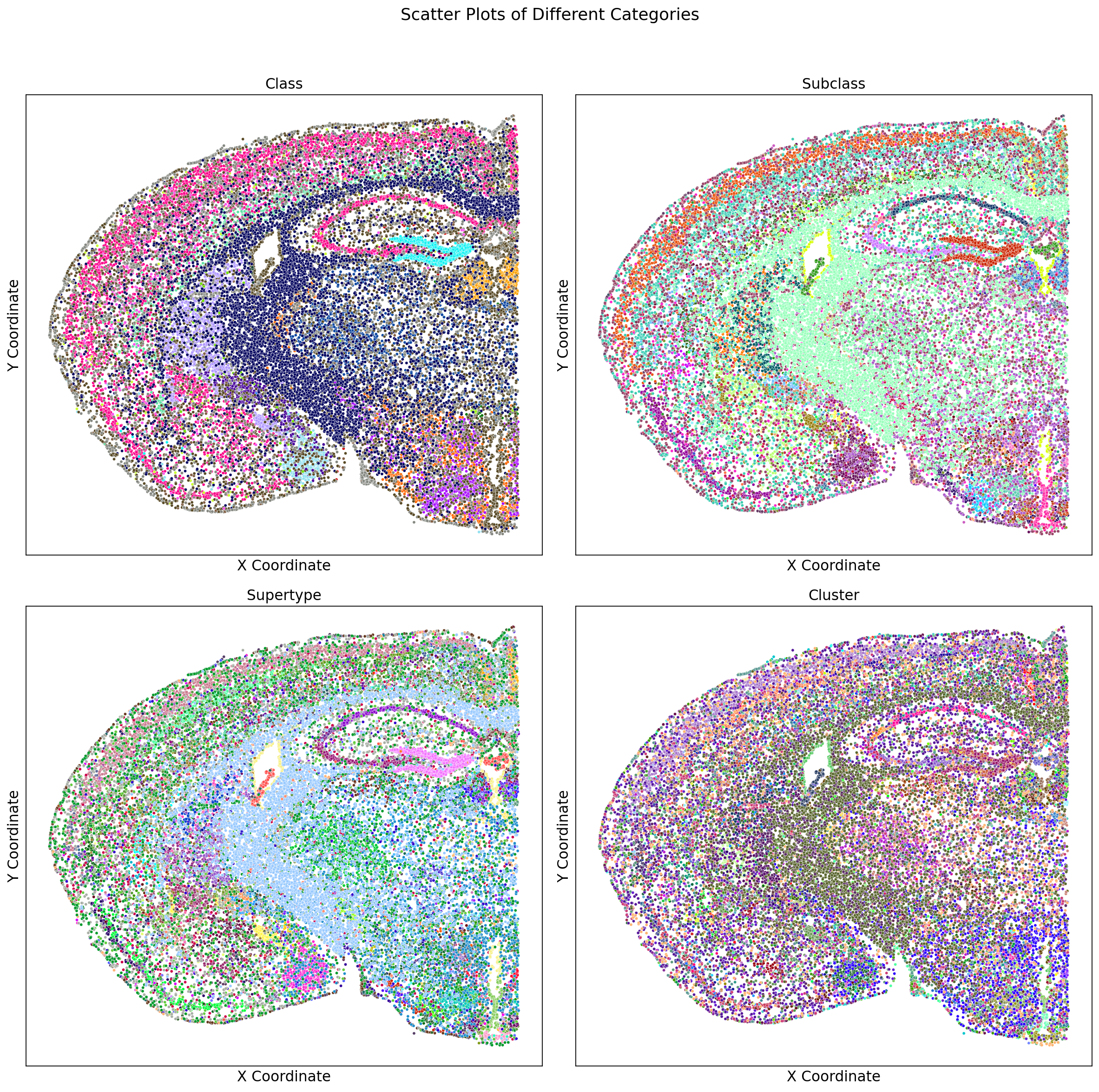
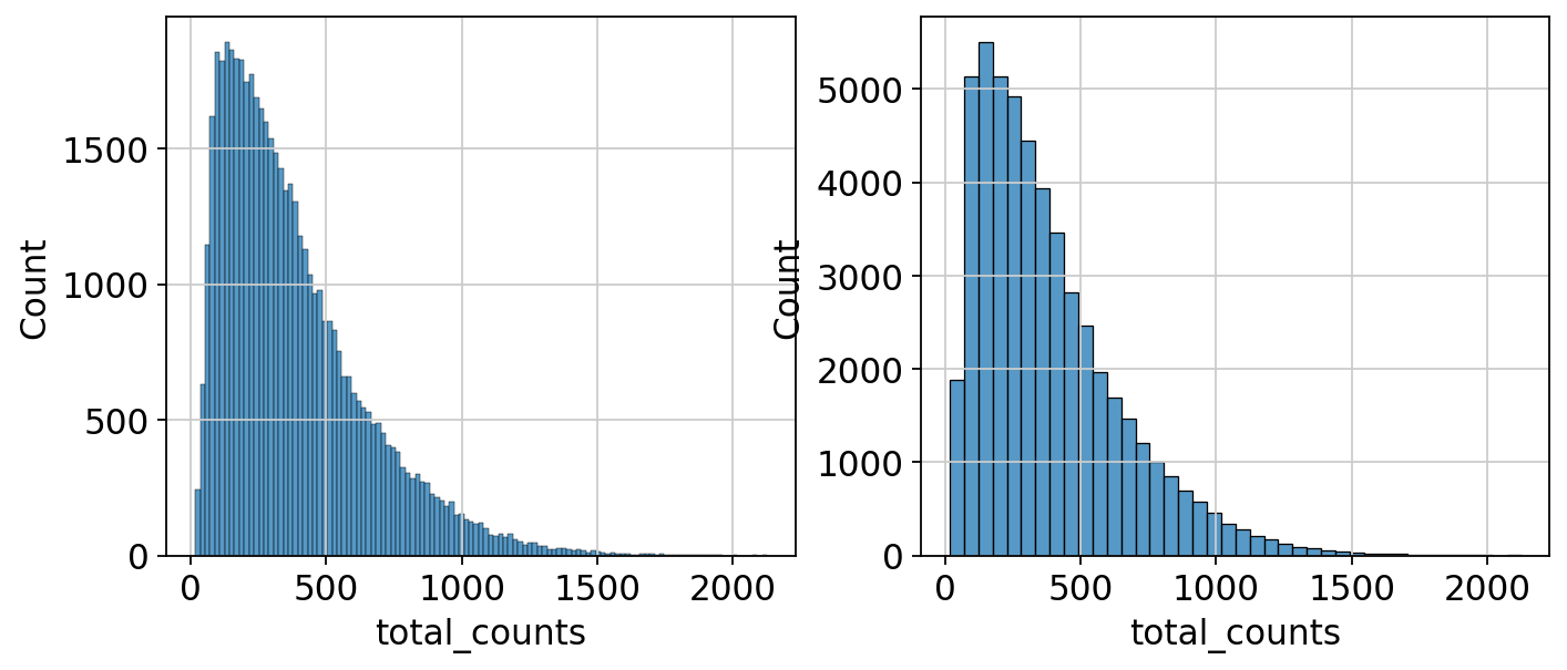
Quality Control
From https://scanpy-tutorials.readthedocs.io/en/latest/spatial/basic-analysis.html
# make gene names unique
adata_section.var_names_make_unique()
# add mt percentage
adata_section.var["mt"] = adata_section.var_names.str.startswith("MT-")
sc.pp.calculate_qc_metrics(adata_section, qc_vars=["mt"], inplace=True)
fig, axs = plt.subplots(1, 2, figsize=(10, 4))
sns.histplot(adata_section.obs["total_counts"], kde=False, ax=axs[0])
sns.histplot(
adata_section.obs["total_counts"][adata_section.obs["total_counts"] < 10000],
kde=False,
bins=40,
ax=axs[1],
)
Cell Filtering and Preprocessing in Single-Cell RNA-Seq Analysis
In this section, we are performing a series of filtering steps to preprocess the single-cell RNA sequencing (scRNA-seq) data stored in the adata_section object. The filtering aims to retain high-quality cells and genes for downstream analyses. The following steps are applied:
- Filter Cells by Minimum Counts:
- We filter out cells that have fewer than 200 counts. This helps to exclude low-quality cells that may not provide reliable information.
sc.pp.filter_cells(adata_section, min_counts=200)- Filter Cells by Maximum Counts:
- We also filter out cells with more than 25,000 counts to remove potential doublets or outlier cells that may artificially inflate the count data
## sol
sc.pp.filter_cells(adata_section, max_counts=25000) ### EX
Filter Based on Mitochondrial Gene Expression:
- We further refine our dataset by excluding cells that have more than 10% of their total counts coming from mitochondrial genes.
adata_section = adata_section[adata_section.obs["pct_counts_mt"] < 10].copy()- Filter Genes by Minimum Cells:
- Finally, we filter out genes that are detected in fewer than 20 cells, ensuring that we retain only those genes that have sufficient expression across our dataset.
Filter out genes that are detected in less than 20 cells
### Hint: use sc.pp.filter_genes
### SOL
sc.pp.filter_genes(adata_section, min_cells=20) print(f"Number of cells after filtering: {adata_section.n_obs}")Number of cells after filtering: 36206Perform PCA and UMAP and cluster with Leiden Algorithm
sc.pp.pca(adata_section)
sc.pp.neighbors(adata_section)
sc.tl.umap(adata_section)
sc.tl.leiden(
    adata_section,
    key_added="clusters",
    resolution=1.0,
    directed=False,
    n_iterations=2
)plt.rcParams["figure.figsize"] = (8,8)
sc.pl.umap(adata_section, color=["total_counts", "n_genes_by_counts", "clusters"], wspace=0.2)
Some stats:
print('Number of Neurotransmitters: ', len(adata_section.obs['neurotransmitter'].unique()))
print('Number of Classes: ', len(adata_section.obs['class'].unique()))
print('Number of Subclasses: ', len(adata_section.obs['subclass'].unique()))
print('Number of Supertype: ', len(adata_section.obs['supertype'].unique()))
print('Number of Cluster: ', len(adata_section.obs['cluster'].unique()))
Number of Neurotransmitters: 7
Number of Classes: 25
Number of Subclasses: 136
Number of Supertype: 420
Number of Cluster: 1000The filtering step performed by the authors of the paper is donw differently than the basic one we just performed. The metadata is given only for the filtered object. For this reason we will filter our object to keep only spots that passed the quality control for the Allen Brain Atlas standards.
# filter spots in adata_section and keep only the ones that are present in metadata
adata_section = adata[adata.obs.index.isin(cell_metadata_extended_sub.index)]
# reindex cell_metadata_ext_sub to match the index order of adata_section.obs
cell_metadata_extended_sub = cell_metadata_extended_sub.reindex(adata_section.obs.index)
# add metadata to the metadata field in an anndata object : adata.obj
adata_section.obs = cell_metadata_extended_sub

print(f"The filtered Section 80 dataset has {adata_section.shape[0]} cells and {adata_section.shape[1]} genes.")
The filtered Section 80 dataset has 37068 cells and 1122 genes. Some spatial tools require the spatial coordinates ti be stored in .obsm as spatial or X_spatial
This is how you can add them:
# add X_spatial
adata_section.obsm['X_spatial'] = np.array(adata_section.obs[['x','y']])
adata_section.obsm['X_spatial']
array([[5.87382373, 1.24637434],
[5.0668137 , 1.21544436],
[4.68106119, 1.28715849],
...,
[0.97304079, 4.80513099],
[0.86566165, 4.29416095],
[0.84111779, 3.8952338 ]]) Once the spatial coordinates are stored in .obsm[X_spatial] you can plot the section with sc.pl.spatial
# Generate the spatial plot
sc.pl.spatial(adata_section, color='class', color_map='Accent_r', spot_size=0.04, title='Section 80 colored by Class')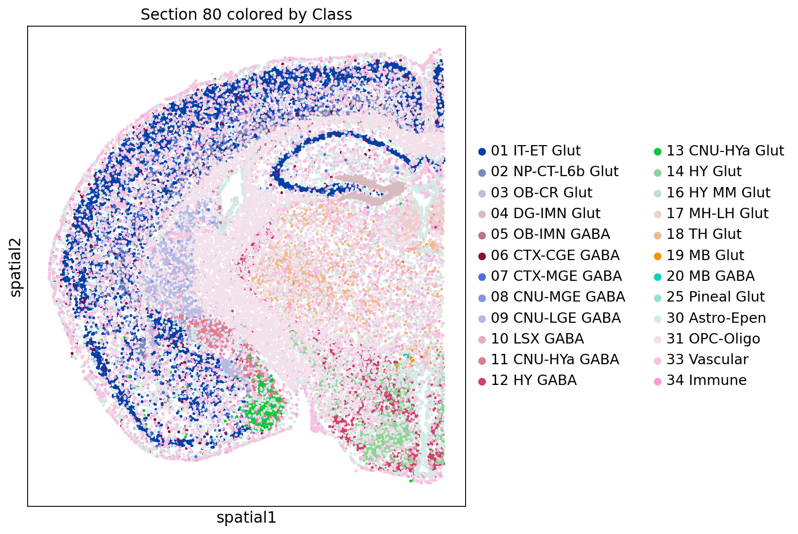
Plot gene expression in space
Since each spot in the spatial data corresponds to a specific location and its associated gene expression profile, we can visualize spatial gene expression.
We can do this using the function sc.pl.spatial, it requires the name of the variable index to indicate the genes to plot.
Let’s take a look at adata_section.var:
adata_section.var.head()| gene_symbol | name | mapped_ncbi_identifier | |
|---|---|---|---|
| gene_identifier | |||
| ENSMUSG00000024798 | Htr7 | 5-hydroxytryptamine (serotonin) receptor 7 | NCBIGene:15566 |
| ENSMUSG00000042385 | Gzmk | granzyme K | NCBIGene:14945 |
| ENSMUSG00000036198 | Arhgap36 | Rho GTPase activating protein 36 | NCBIGene:75404 |
| ENSMUSG00000028780 | Sema3c | sema domain, immunoglobulin domain (Ig), short... | NCBIGene:20348 |
| ENSMUSG00000015843 | Rxrg | retinoid X receptor gamma | NCBIGene:20183 |
Change the index of the adata_section.var to gene_symbol for clarity
# Reset the index to turn the current index into a column
adata_section.var.reset_index(inplace=True)
adata_section.var.set_index('gene_symbol', inplace=True)
adata_section.var.head()| gene_identifier | name | mapped_ncbi_identifier | |
|---|---|---|---|
| gene_symbol | |||
| Htr7 | ENSMUSG00000024798 | 5-hydroxytryptamine (serotonin) receptor 7 | NCBIGene:15566 |
| Gzmk | ENSMUSG00000042385 | granzyme K | NCBIGene:14945 |
| Arhgap36 | ENSMUSG00000036198 | Rho GTPase activating protein 36 | NCBIGene:75404 |
| Sema3c | ENSMUSG00000028780 | sema domain, immunoglobulin domain (Ig), short... | NCBIGene:20348 |
| Rxrg | ENSMUSG00000015843 | retinoid X receptor gamma | NCBIGene:20183 |
# Define genes to plot
genes_toplot = ['Zic1',
 'Penk',
 'Gfap',
 'Dlx6',
 'Cux2',
 'Fezf2',
 'Eomes',
 'Bcl11b',
 'Reln',
 'Nr4a2',
 'Satb2']

sc.pl.spatial(adata_section, color=genes_toplot,spot_size=0.04)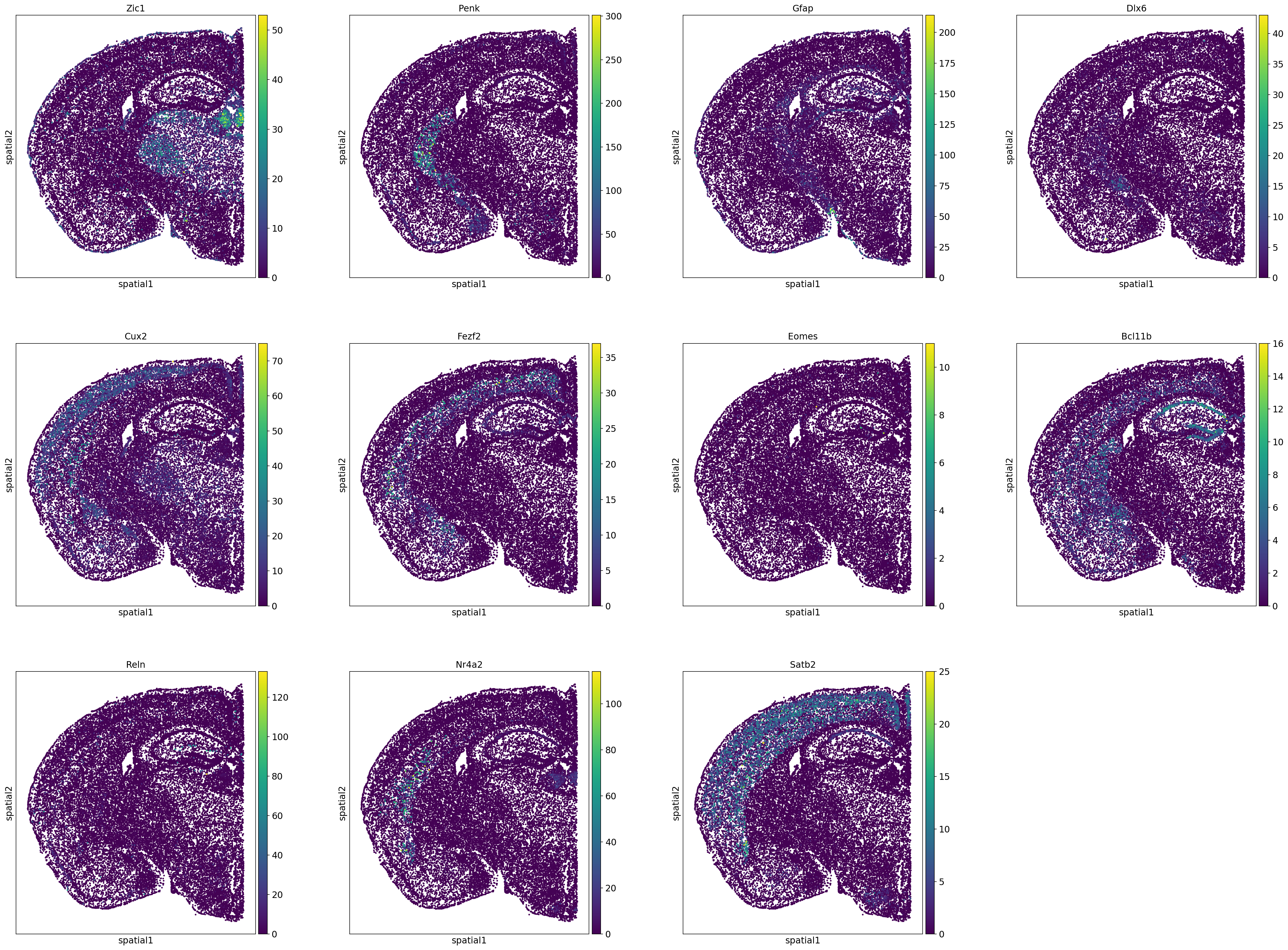
Plot your favourite gene/s
genes_toplot = [.....]

sc.pl.spatial(adata_section, color=genes_toplot,spot_size=0.04)adata_section.write_h5ad('adata_section80.h5ad')# Record the end time
end_time = time.time()
# Calculate elapsed time in minutes
elapsed_time = (end_time - start_time) / 60
print(f"Execution Time: {elapsed_time:.2f} minutes")Execution Time: 7.71 minutesPrediction of spatial patterns for unmeasured genes using scRNA-seq data with SpaGE
start_time = time.time()from SpaGE.main import SpaGE
import scipy.stats as st
SpaGE takes as input the (targeted) spatial dataset (query) and a single-cell RNA dataset used as reference. The two datasets should be generated under the same conditions (same species, tissue, region) as much as possible.
We will use Mouse whole-brain transcriptomic cell type atlas (Hongkui Zeng).This scRNAseq dataset profiled 7 million cells (approximately 4.0 million cells passing quality control). More in detail:
1.7 million single cell transcriptomes spanning the whole adult mouse brain using 10Xv2 chemistry (WMB-10Xv2)
2.3 million single cell transcriptomes spanning the whole adult mouse brain using 10Xv3 chemistry (WMB-10Xv3)
1687 single cell transcriptomes spanning the whole adult mouse brain using the 10X Multiome chemistry (WMB-10XMulti)

Let’s check the names of the files in each of the three single-cell collections:
abc_cache.list_data_files('WMB-10Xv2')['WMB-10Xv2-CTXsp/log2',
'WMB-10Xv2-CTXsp/raw',
'WMB-10Xv2-HPF/log2',
'WMB-10Xv2-HPF/raw',
'WMB-10Xv2-HY/log2',
'WMB-10Xv2-HY/raw',
'WMB-10Xv2-Isocortex-1/log2',
'WMB-10Xv2-Isocortex-1/raw',
'WMB-10Xv2-Isocortex-2/log2',
'WMB-10Xv2-Isocortex-2/raw',
'WMB-10Xv2-Isocortex-3/log2',
'WMB-10Xv2-Isocortex-3/raw',
'WMB-10Xv2-Isocortex-4/log2',
'WMB-10Xv2-Isocortex-4/raw',
'WMB-10Xv2-MB/log2',
'WMB-10Xv2-MB/raw',
'WMB-10Xv2-OLF/log2',
'WMB-10Xv2-OLF/raw',
'WMB-10Xv2-TH/log2',
'WMB-10Xv2-TH/raw']abc_cache.list_data_files('WMB-10Xv3')['WMB-10Xv3-CB/log2',
'WMB-10Xv3-CB/raw',
'WMB-10Xv3-CTXsp/log2',
'WMB-10Xv3-CTXsp/raw',
'WMB-10Xv3-HPF/log2',
'WMB-10Xv3-HPF/raw',
'WMB-10Xv3-HY/log2',
'WMB-10Xv3-HY/raw',
'WMB-10Xv3-Isocortex-1/log2',
'WMB-10Xv3-Isocortex-1/raw',
'WMB-10Xv3-Isocortex-2/log2',
'WMB-10Xv3-Isocortex-2/raw',
'WMB-10Xv3-MB/log2',
'WMB-10Xv3-MB/raw',
'WMB-10Xv3-MY/log2',
'WMB-10Xv3-MY/raw',
'WMB-10Xv3-OLF/log2',
'WMB-10Xv3-OLF/raw',
'WMB-10Xv3-P/log2',
'WMB-10Xv3-P/raw',
'WMB-10Xv3-PAL/log2',
'WMB-10Xv3-PAL/raw',
'WMB-10Xv3-STR/log2',
'WMB-10Xv3-STR/raw',
'WMB-10Xv3-TH/log2',
'WMB-10Xv3-TH/raw']abc_cache.list_data_files('WMB-10XMulti')['WMB-10XMulti/log2', 'WMB-10XMulti/raw']Let’s check the size of the files in each of the three single-cell collections:
print(f"Size of WMB-10Xv2 data: {abc_cache.get_directory_data_size('WMB-10Xv2')}")Size of WMB-10Xv2 data: 104.16 GBprint(f"Size of WMB-10Xv3 data: {abc_cache.get_directory_data_size('WMB-10Xv3')}")Size of WMB-10Xv3 data: 176.41 GBprint(f"Size of WMB-10X Multi data: {abc_cache.get_directory_data_size('WMB-10XMulti')}")Size of WMB-10X Multi data: 211.28 MB The size is of the combined single-cell object is around 280GB. For this reason, the three objects have been previously downloaded, concatenated, preprocessed and subsetted to obtain NNN cells. For your knowledge, you can find all the steps in obtain_scref.py.
Let’s read the resulting single-cell AnnData object:
wd = '/exports/humgen/bmanzato/spatial_workshop'

adata_sc = ad.read_h5ad('/exports/humgen/bmanzato/spatial_workshop/sc_adata_1percent.h5ad')
Inspect the object:
adata_scAnnData object with n_obs × n_vars = 28981 × 32285
obs: 'cell_barcode', 'barcoded_cell_sample_label', 'library_label', 'feature_matrix_label', 'entity', 'brain_section_label', 'library_method', 'region_of_interest_acronym', 'donor_label', 'donor_genotype', 'donor_sex', 'dataset_label', 'x', 'y', 'cluster_alias'Inspect the metadata:
adata_sc.obs.head()| cell_barcode | barcoded_cell_sample_label | library_label | feature_matrix_label | entity | brain_section_label | library_method | region_of_interest_acronym | donor_label | donor_genotype | donor_sex | dataset_label | x | y | cluster_alias | |
|---|---|---|---|---|---|---|---|---|---|---|---|---|---|---|---|
| cell_label | |||||||||||||||
| GTATTCTCAGCTATTG-045_C01 | GTATTCTCAGCTATTG | 045_C01 | L8TX_180829_01_C10 | WMB-10Xv2-TH | cell | NaN | 10Xv2 | TH | Snap25-IRES2-Cre;Ai14-407905 | Snap25-IRES2-Cre/wt;Ai14(RCL-tdT)/wt | F | WMB-10Xv2 | 12.420248 | -10.367616 | 5076 |
| GTGTGATCACCAGCGT-468_A02 | GTGTGATCACCAGCGT | 468_A02 | L8TX_201217_01_D07 | WMB-10Xv3-MB | cell | NaN | 10Xv3 | MB | Snap25-IRES2-Cre;Ai14-556231 | Ai14(RCL-tdT)/wt | F | WMB-10Xv3 | 1.571478 | 23.592803 | 14956 |
| TAACCAGCACCAAATC-204.2_A01 | TAACCAGCACCAAATC | 204.2_A01 | L8TX_200122_01_F12 | WMB-10Xv3-MB | cell | NaN | 10Xv3 | MB | Snap25-IRES2-Cre;Ai14-504535 | Snap25-IRES2-Cre/wt;Ai14(RCL-tdT)/wt | F | WMB-10Xv3 | -12.491472 | 11.322906 | 5231 |
| AGCGTCGGTTCAGCGC-420_C06 | AGCGTCGGTTCAGCGC | 420_C06 | L8TX_201106_01_G03 | WMB-10Xv3-MB | cell | NaN | 10Xv3 | MB | Snap25-IRES2-Cre;Ai14-551017 | Ai14(RCL-tdT)/wt | M | WMB-10Xv3 | -10.406498 | 11.711900 | 5230 |
| AGACAAAAGAACTCCT-278_B03 | AGACAAAAGAACTCCT | 278_B03 | L8TX_200702_01_H01 | WMB-10Xv3-TH | cell | NaN | 10Xv3 | TH | Snap25-IRES2-Cre;Ai14-529474 | Snap25-IRES2-Cre/wt;Ai14(RCL-tdT)/wt | F | WMB-10Xv3 | 5.455338 | -13.476950 | 5101 |
Add feature metadata to the AnnData object
genes = pd.read_csv('/exports/humgen/bmanzato/abc_download_root/metadata/WMB-10X/20231215/gene.csv',index_col=0)
genes.head()| gene_symbol | name | mapped_ncbi_identifier | comment | |
|---|---|---|---|---|
| gene_identifier | ||||
| ENSMUSG00000051951 | Xkr4 | X-linked Kx blood group related 4 | NCBIGene:497097 | NaN |
| ENSMUSG00000089699 | Gm1992 | predicted gene 1992 | NaN | NaN |
| ENSMUSG00000102331 | Gm19938 | predicted gene, 19938 | NaN | NaN |
| ENSMUSG00000102343 | Gm37381 | predicted gene, 37381 | NaN | NaN |
| ENSMUSG00000025900 | Rp1 | retinitis pigmentosa 1 (human) | NCBIGene:19888 | NaN |
adata_sc.var = genes# Reset the index to turn the current index into a column
adata_sc.var.reset_index(inplace=True)
adata_sc.var.set_index('gene_symbol', inplace=True)
adata_sc.var.head()| gene_identifier | name | mapped_ncbi_identifier | comment | |
|---|---|---|---|---|
| gene_symbol | ||||
| Xkr4 | ENSMUSG00000051951 | X-linked Kx blood group related 4 | NCBIGene:497097 | NaN |
| Gm1992 | ENSMUSG00000089699 | predicted gene 1992 | NaN | NaN |
| Gm19938 | ENSMUSG00000102331 | predicted gene, 19938 | NaN | NaN |
| Gm37381 | ENSMUSG00000102343 | predicted gene, 37381 | NaN | NaN |
| Rp1 | ENSMUSG00000025900 | retinitis pigmentosa 1 (human) | NCBIGene:19888 | NaN |
Set up inputs for SpaGE:
# Extract the count data and transform them into a Pandas DataFrame
RNA_data = pd.DataFrame(adata_sc.X.todense())
# Add gene names to the RNA_data columns
RNA_data.columns = adata_sc.var.index# Filter lowely expressed genes
Genes_count = np.sum(RNA_data > 0, axis=1)
RNA_data = RNA_data.loc[Genes_count >=10,:]
del Genes_count# Normalization
def Log_Norm_cpm(x):
return np.log(((x/np.sum(x))*1000000) + 1)
RNA_data = RNA_data.apply(Log_Norm_cpm,axis=0)# transpose RNA_data to have rows = genes and columns = cells
RNA_data = RNA_data.TRNA_data.head()| 0 | 1 | 2 | 3 | 4 | 5 | 6 | 7 | 8 | 9 | ... | 28971 | 28972 | 28973 | 28974 | 28975 | 28976 | 28977 | 28978 | 28979 | 28980 | |
|---|---|---|---|---|---|---|---|---|---|---|---|---|---|---|---|---|---|---|---|---|---|
| gene_symbol | |||||||||||||||||||||
| Xkr4 | 4.552345 | 0.0 | 4.130508 | 0.0 | 5.504673 | 2.214984 | 2.583386 | 3.238043 | 2.214984 | 3.911375 | ... | 0.0 | 4.673730 | 4.253778 | 2.583386 | 3.733048 | 4.673730 | 0.0 | 0.0 | 2.852008 | 2.583386 |
| Gm1992 | 0.000000 | 0.0 | 0.000000 | 0.0 | 0.000000 | 0.000000 | 0.000000 | 0.000000 | 0.000000 | 5.087625 | ... | 0.0 | 6.182114 | 0.000000 | 0.000000 | 0.000000 | 5.087625 | 0.0 | 0.0 | 0.000000 | 0.000000 |
| Gm19938 | 4.665658 | 0.0 | 0.000000 | 0.0 | 5.354088 | 0.000000 | 0.000000 | 0.000000 | 0.000000 | 5.576285 | ... | 0.0 | 5.067980 | 3.981880 | 4.665658 | 0.000000 | 3.981880 | 0.0 | 0.0 | 0.000000 | 3.981880 |
| Gm37381 | 0.000000 | 0.0 | 0.000000 | 0.0 | 0.000000 | 0.000000 | 0.000000 | 0.000000 | 0.000000 | 0.000000 | ... | 0.0 | 0.000000 | 0.000000 | 0.000000 | 0.000000 | 0.000000 | 0.0 | 0.0 | 0.000000 | 0.000000 |
| Rp1 | 0.000000 | 0.0 | 0.000000 | 0.0 | 0.000000 | 0.000000 | 0.000000 | 0.000000 | 0.000000 | 0.000000 | ... | 0.0 | 0.000000 | 0.000000 | 0.000000 | 0.000000 | 0.000000 | 0.0 | 0.0 | 0.000000 | 0.000000 |
5 rows × 28981 columns
# Drop any row with at least one NaN value
RNA_data = RNA_data.dropna()  # This will drop any row with at least one NaN value
How many genes do the spatial and single-cell data set have in common?
## Hint: use .intersection
## SOL
gene_intersection = set(list(adata_section.var.index)).intersection(set(list(adata_sc.var.index)))
len(gene_intersection)1122How many genes are measured in the single-cell dataset that are not measured in the spatial dataset?
##
## SOL
genes_not_intersection = list(set(RNA_data.index) - set(adata_section.var.index))
len(genes_not_intersection)27078# Extract count matrix from adata_section and rename index and column names
spatial_data = pd.DataFrame(adata_section.X)
spatial_data.index = adata_section.obs.index
spatial_data.columns = adata_section.var.index# Normalize spatial_data
spatial_data = spatial_data.apply(Log_Norm_cpm,axis=0)brain_region_specific_genes = [
"Bcl11b", "Cux2", "Fezf2", "Tbr1", "Satb2", # isocortex
"Nr4a2", # Midbrain specific
"Foxp2", # Striatum specific
"Penk", # Basal ganglia specific
"Zic1", # Cerebellum specific
"Hoxb2", # Hindbrain specific
"Dlx6", # Subpallium specific
"Reln", # Hippocampus specific
"Gfap" # Astrocytes in multiple brain regions
]
# Checking for overlap
overlap_genes = list(set(list(spatial_data.columns)) & set(brain_region_specific_genes))
overlap_genes['Reln',
'Fezf2',
'Bcl11b',
'Nr4a2',
'Zic1',
'Penk',
'Dlx6',
'Cux2',
'Satb2',
'Gfap']# non overlap genes
non_overlap_genes = list(set(brain_region_specific_genes) - set(overlap_genes))Leave-one-gene-out cross validation
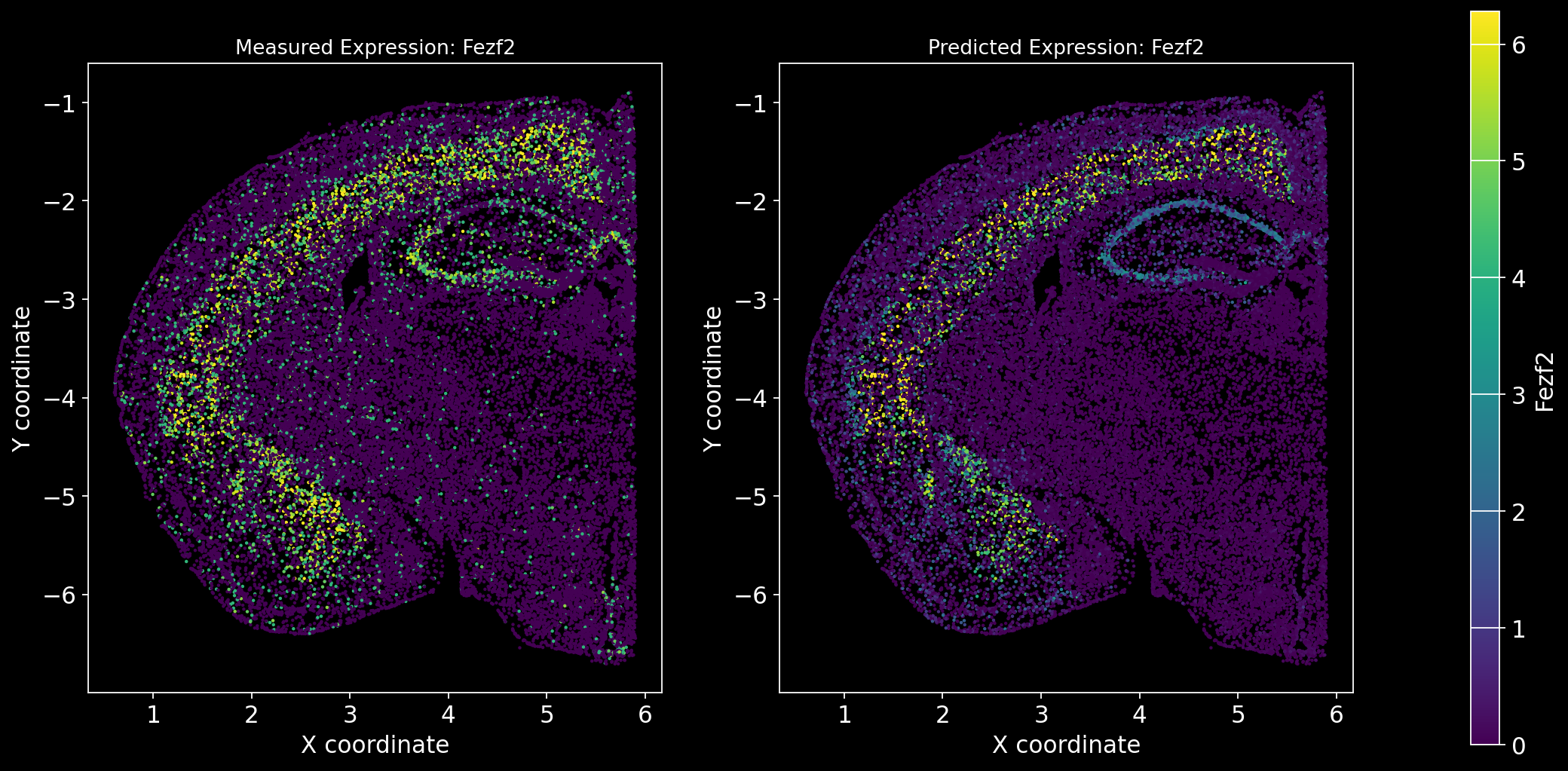
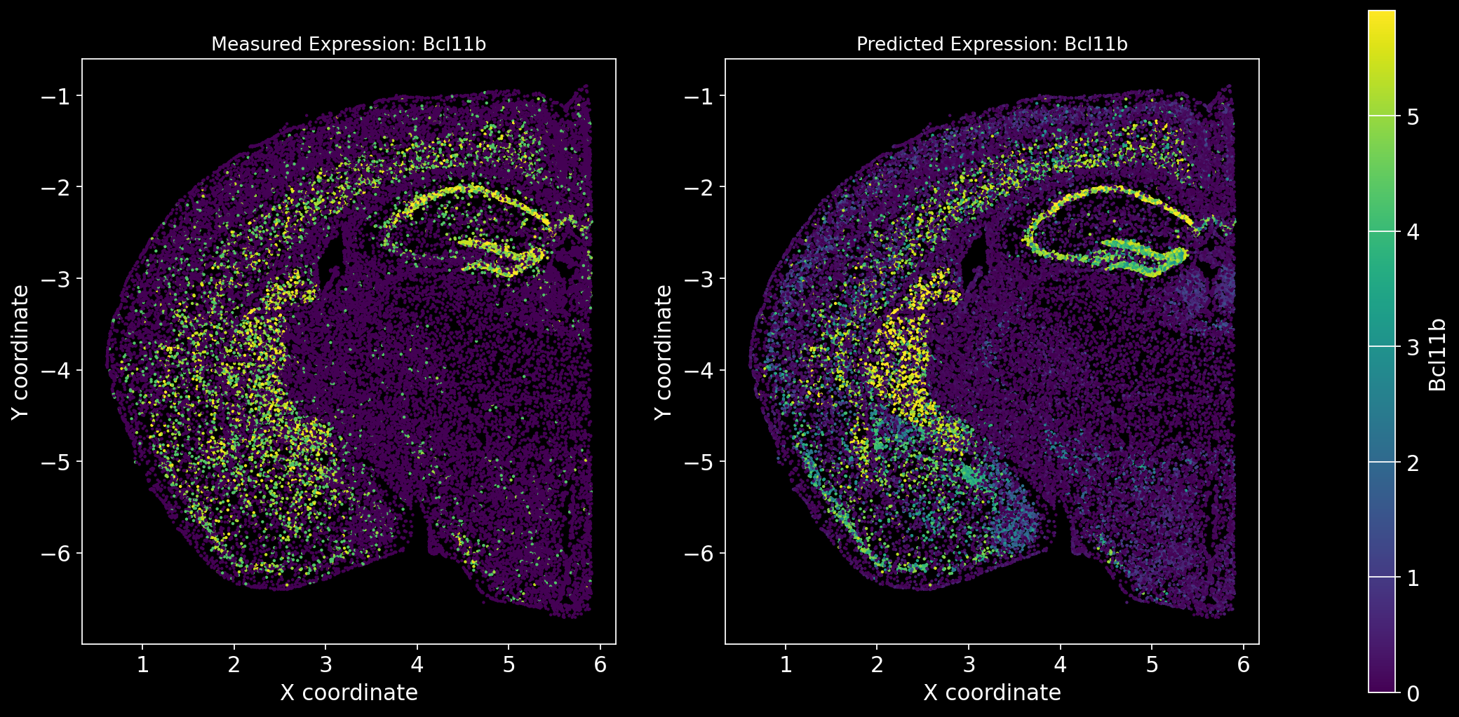
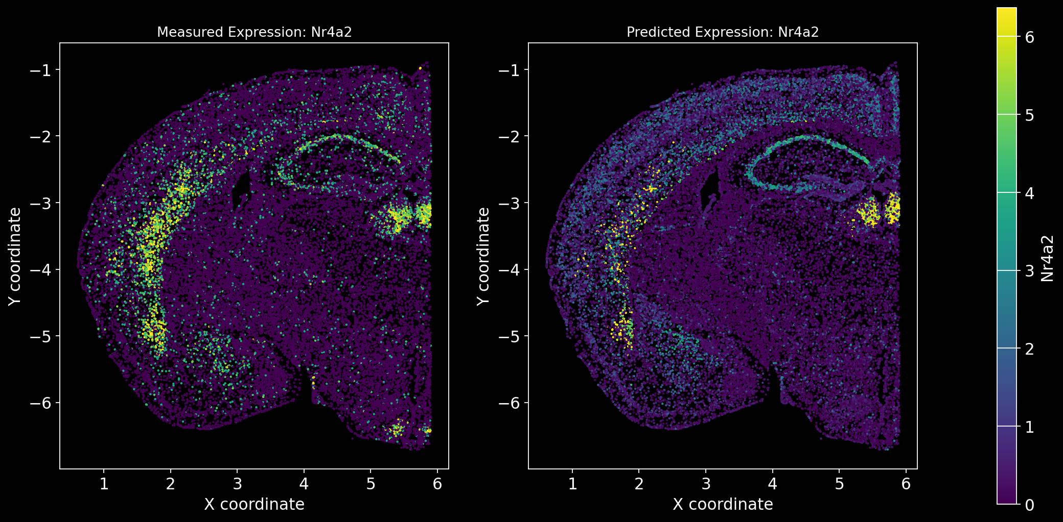
Define the function to predict genes measured in the spatial dataset to have a ground truth and plot the measured expression next to the predicted one. Calculate Spearman correlation between the measured and predicted expression.
import matplotlib.gridspec as gridspec  # Import for more precise subplot layout control
plt.style.use('dark_background')

def plot_measured_predicted(Gene_set):

    for i in Gene_set:
        # Predict the expression of the current gene using the SpaGE method
        Imp_Genes = SpaGE(spatial_data.drop(i, axis=1), RNA_data.T, n_pv=30, genes_to_predict=[i])

        # Calculate the Spearman correlation between measured and predicted values
        Correlations[i] = st.spearmanr(spatial_data[i], Imp_Genes[i])[0]

        # Create a figure with two subplots (1 row, 2 columns)
        fig = plt.figure(figsize=(15, 8))  # Adjust figure size if needed
        gs = gridspec.GridSpec(1, 3, width_ratios=[1, 1, 0.05], wspace=0.3)  # Create a gridspec for better control

        # --- Measured Gene Expression Plot ---
        ax0 = fig.add_subplot(gs[0])  # First plot
        cmap_measured = spatial_data[i]
        cmap_measured[cmap_measured > np.percentile(cmap_measured, 99)] = np.percentile(cmap_measured, 99)
        sc1 = ax0.scatter(adata_section.obs['x'], -adata_section.obs['y'], s=1, c=cmap_measured, alpha=1)

        ax0.set_title(f'Measured Expression: {i}', fontsize=12)
        ax0.set_xlabel('X coordinate')
        ax0.set_ylabel('Y coordinate')
        ax0.set_aspect('equal', adjustable='box')
        ax0.grid(False)

        # --- Predicted Gene Expression Plot ---
        ax1 = fig.add_subplot(gs[1])  # Second plot
        cmap_predicted = Imp_Genes[i]
        cmap_predicted[cmap_predicted > np.percentile(cmap_predicted, 99)] = np.percentile(cmap_predicted, 99)
        sc2 = ax1.scatter(adata_section.obs['x'], -adata_section.obs['y'], s=1, c=cmap_predicted, alpha=1)

        ax1.set_title(f'Predicted Expression: {i}', fontsize=12)
        ax1.set_xlabel('X coordinate')
        ax1.set_ylabel('Y coordinate')
        ax1.set_aspect('equal', adjustable='box')
        ax1.grid(False)

        # Create a colorbar on the far right
        cbar_ax = fig.add_subplot(gs[2])  # Third subplot (narrow space for the color bar)
        cbar = fig.colorbar(sc1, cax=cbar_ax)  # Assign the color bar to the third subplot
        cbar.set_label(i)

        # Show the plot
        plt.tight_layout()  # Adjust spacing to avoid overlap
        plt.show()
# Define the set of genes (from the gene_intersection list) where we will perform leave-one-out cross-validation
Gene_set = overlap_genes
# Since we have a ground truth, create a Series to store Spearman correlation results for each gene
Correlations = pd.Series(index=Gene_set)
plot_measured_predicted(Gene_set)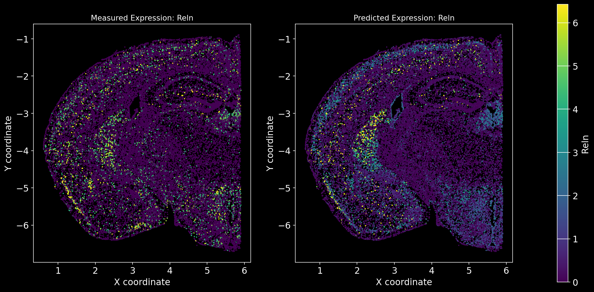
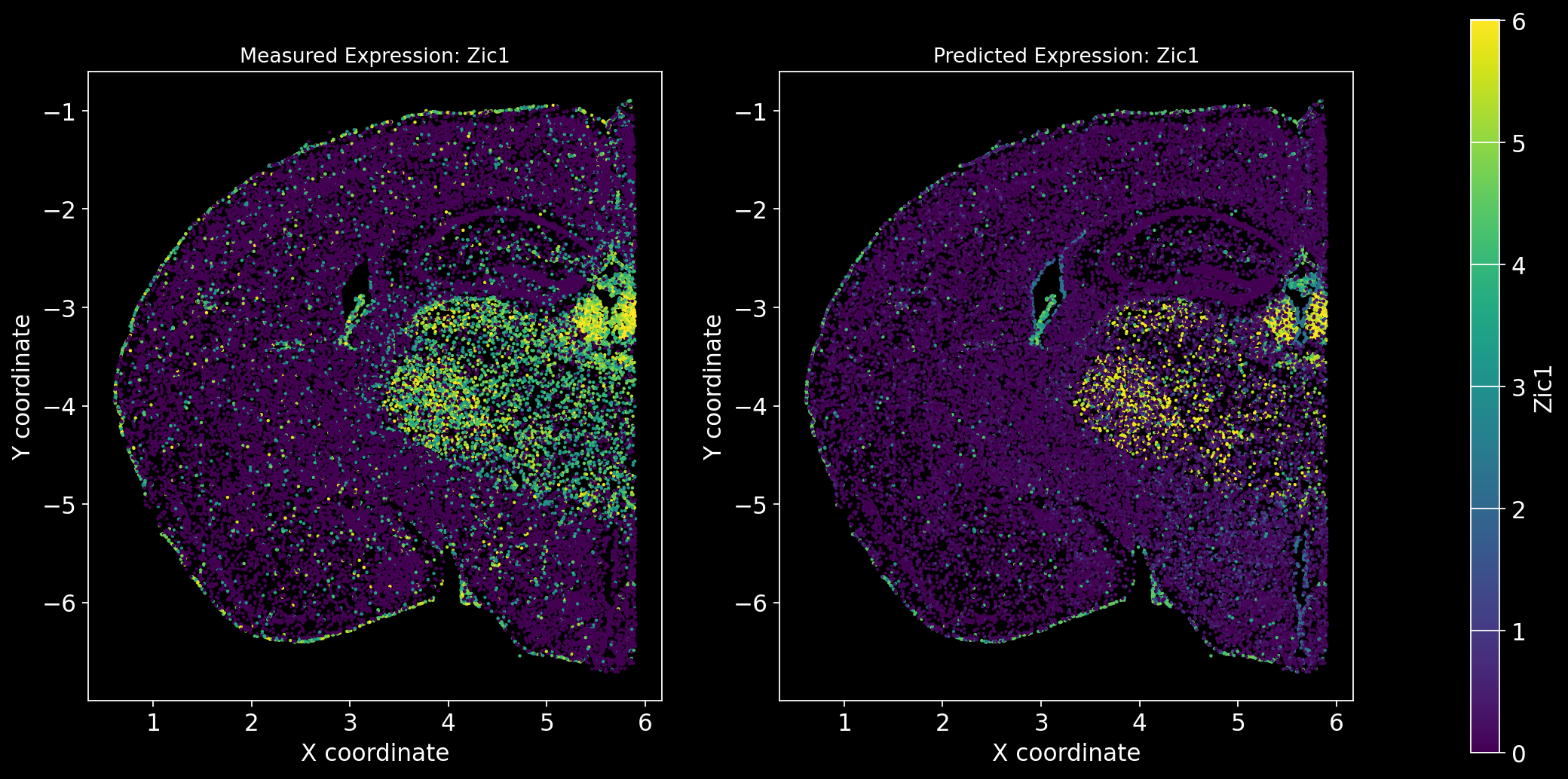
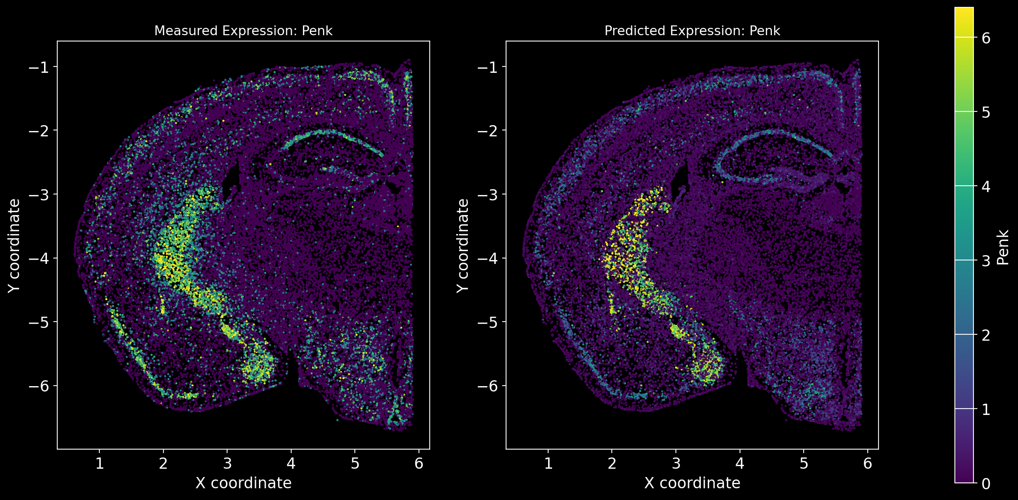
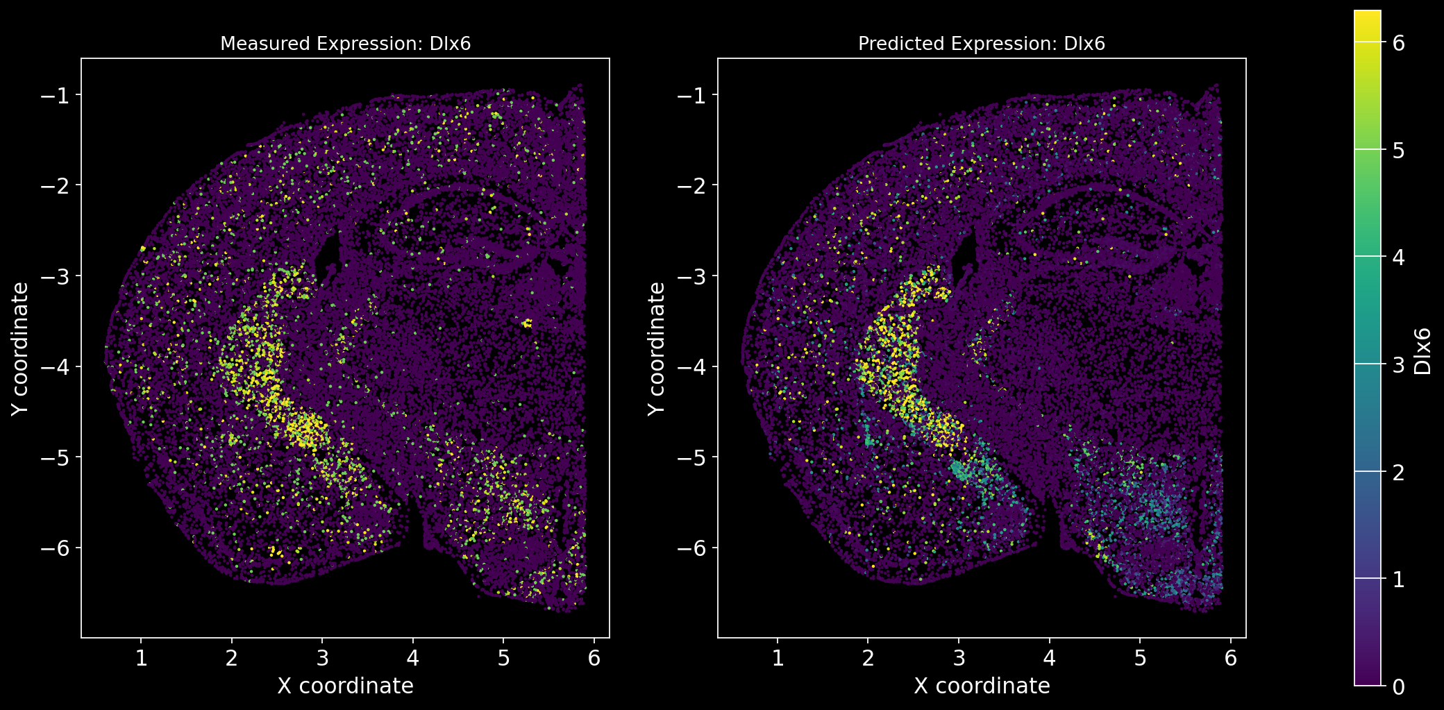
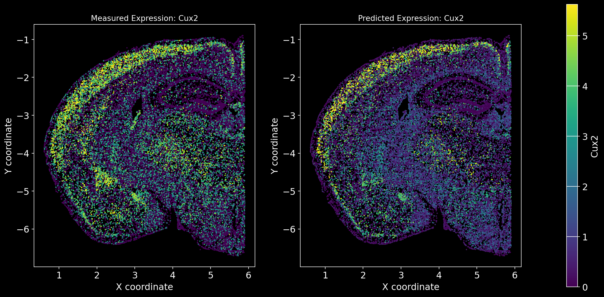
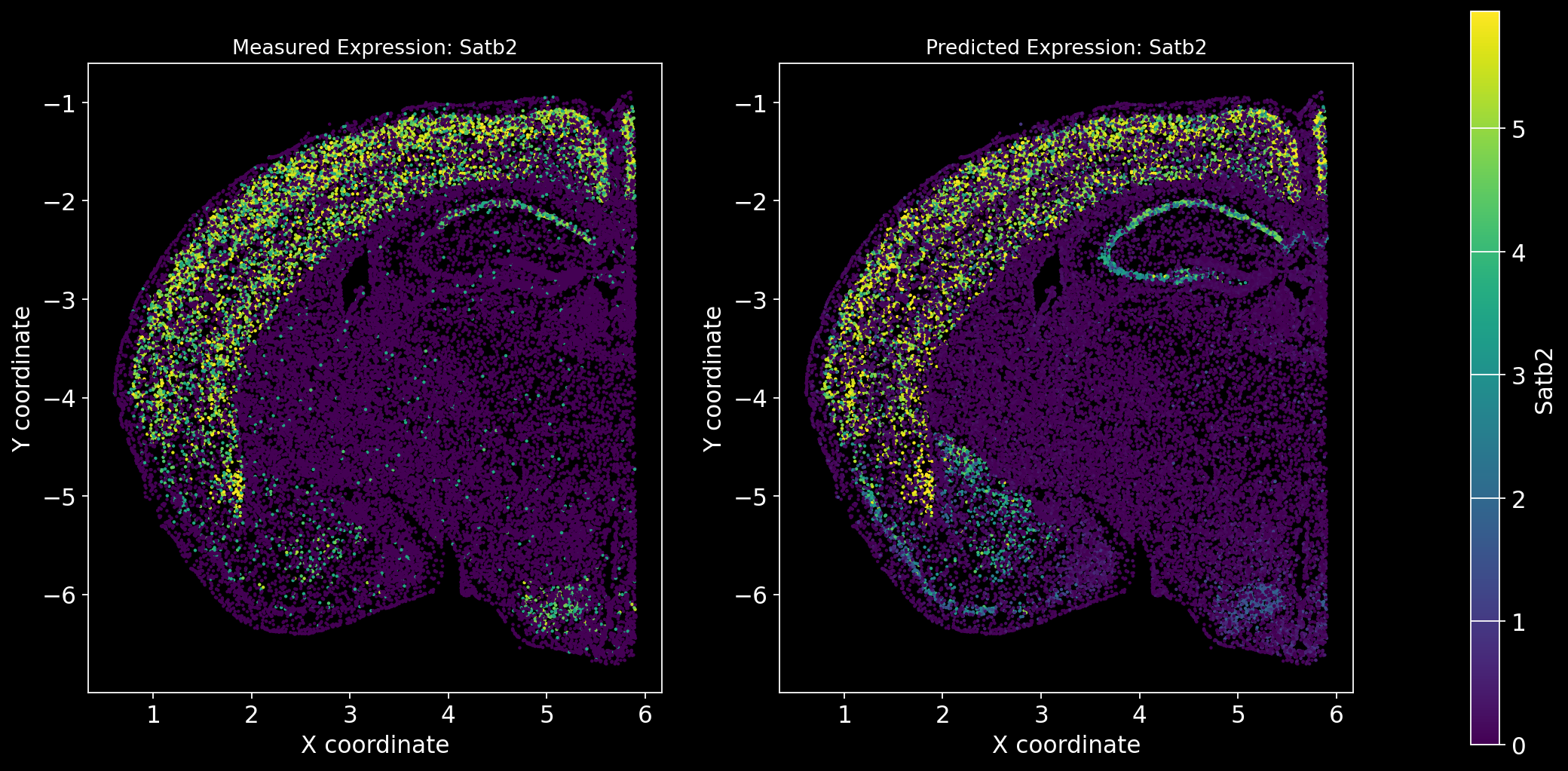
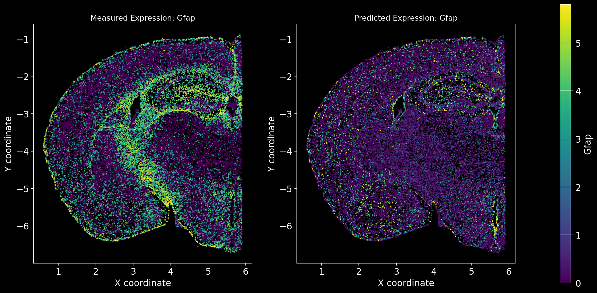
Let’s take a look at the Spearman Correlations between measured and predicted gene expression:
pd.DataFrame(Correlations)| 0 | |
|---|---|
| Reln | 0.330431 |
| Fezf2 | 0.428543 |
| Bcl11b | 0.476758 |
| Nr4a2 | 0.304546 |
| Zic1 | 0.560149 |
| Penk | 0.461395 |
| Dlx6 | 0.402919 |
| Cux2 | 0.623264 |
| Satb2 | 0.570017 |
| Gfap | 0.307733 |
Is there any other gene expression (measured in the spatial dataset) you would like to predict?
# Define the set of genes (from the gene_intersection list) where we will perform leave-one-out cross-validation
Gene_set = ..... # has to be a list
# Since we have a ground truth, create a Series to store Spearman correlation results for each gene
Correlations = pd.Series(index=Gene_set)

plot_measured_predicted(Gene_set)
# print Correlations
pd.DataFrame(Correlations)Predict unmeasured genes
Define a function to predict unmeasured genes in the spatial dataset.
In this case correlations cannot be calculated as there is no ground truth available.
def predict_unmeasured_genes(Gene_set):
    for i in Gene_set:

        # Predict the expression of the current gene using the SpaGE method
        Imp_Genes = SpaGE(spatial_data, RNA_data.T, n_pv=30, genes_to_predict=[i])

        # Create a new figure for each gene's predicted expression
        plt.figure(figsize=(10, 8))

        # Get predicted gene expression values and clip both lower and upper bounds
        cmap_predicted = Imp_Genes[i]

        # Clip the minimum values at 0 (no negatives) and limit extreme values at 99th percentile
        cmap_predicted = np.clip(cmap_predicted, 0, np.percentile(cmap_predicted, 99))

        # Plot scatter plot for the predicted gene expression
        sc2 = plt.scatter(adata_section.obs['x'], -adata_section.obs['y'], s=1, c=cmap_predicted, alpha=1)

        # Set plot title and labels
        plt.title(f'Predicted Expression: {i}', fontsize=12)
        plt.xlabel('X coordinate')
        plt.ylabel('Y coordinate')
        plt.gca().set_aspect('equal', adjustable='box')
        plt.grid(False)

        # Create a colorbar on the same plot
        cbar = plt.colorbar(sc2)
        cbar.set_label(i)

        # Adjust layout and display the plot
        plt.tight_layout()
        plt.show()
# Define the set of genes (from the non_overlap_genes list) to be predicted by SpaGE
Gene_set = non_overlap_genes
predict_unmeasured_genes(Gene_set)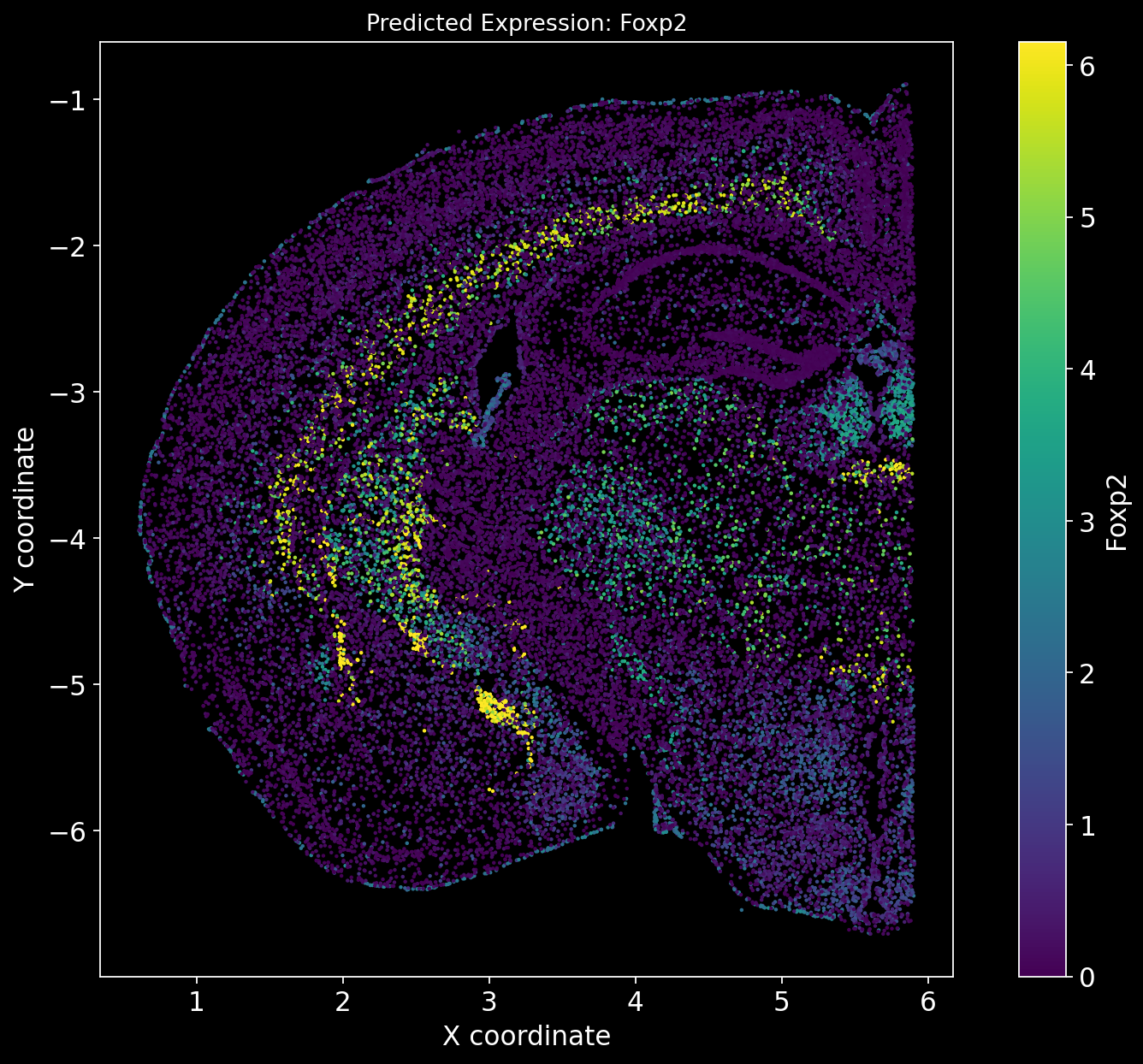
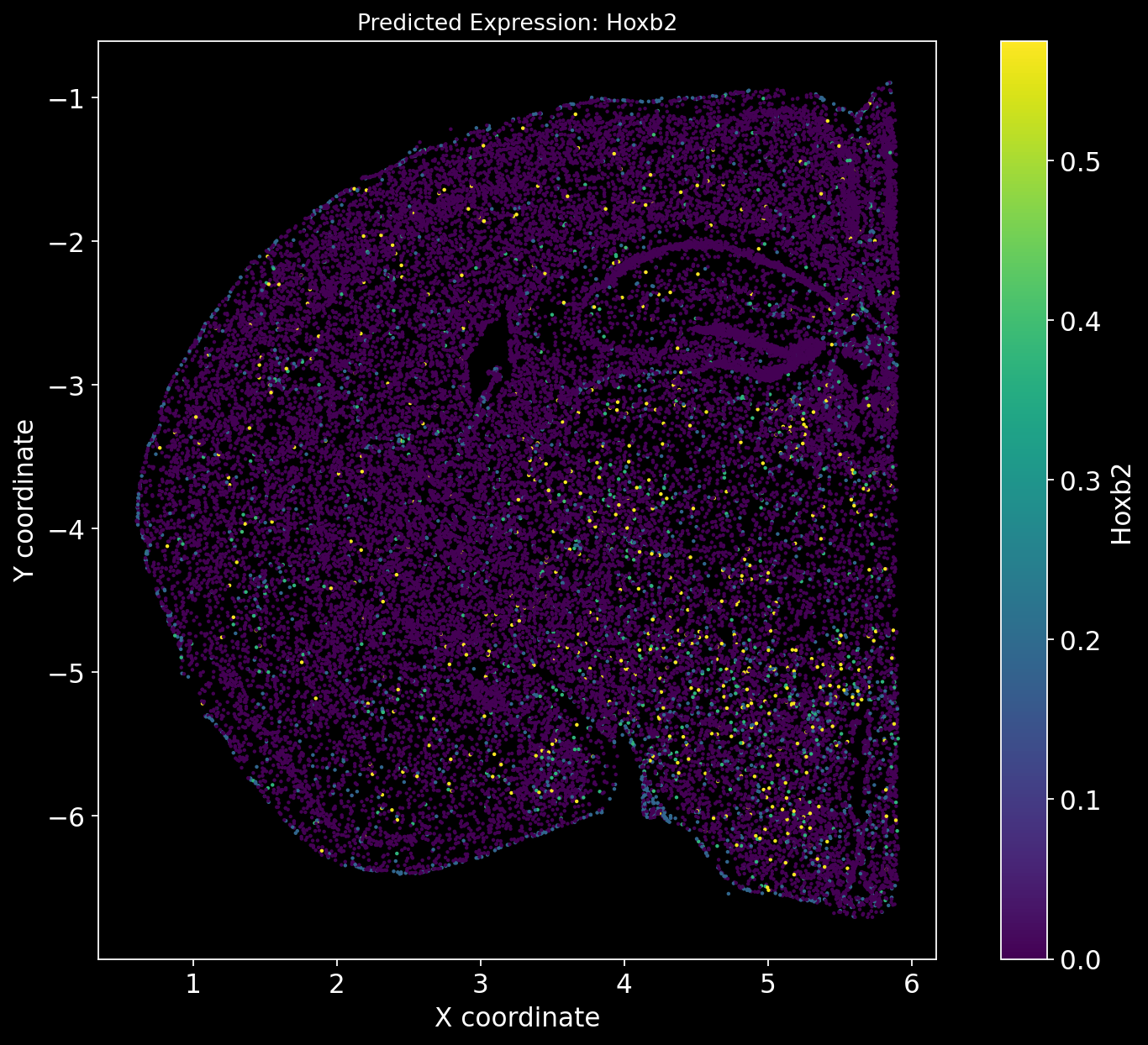
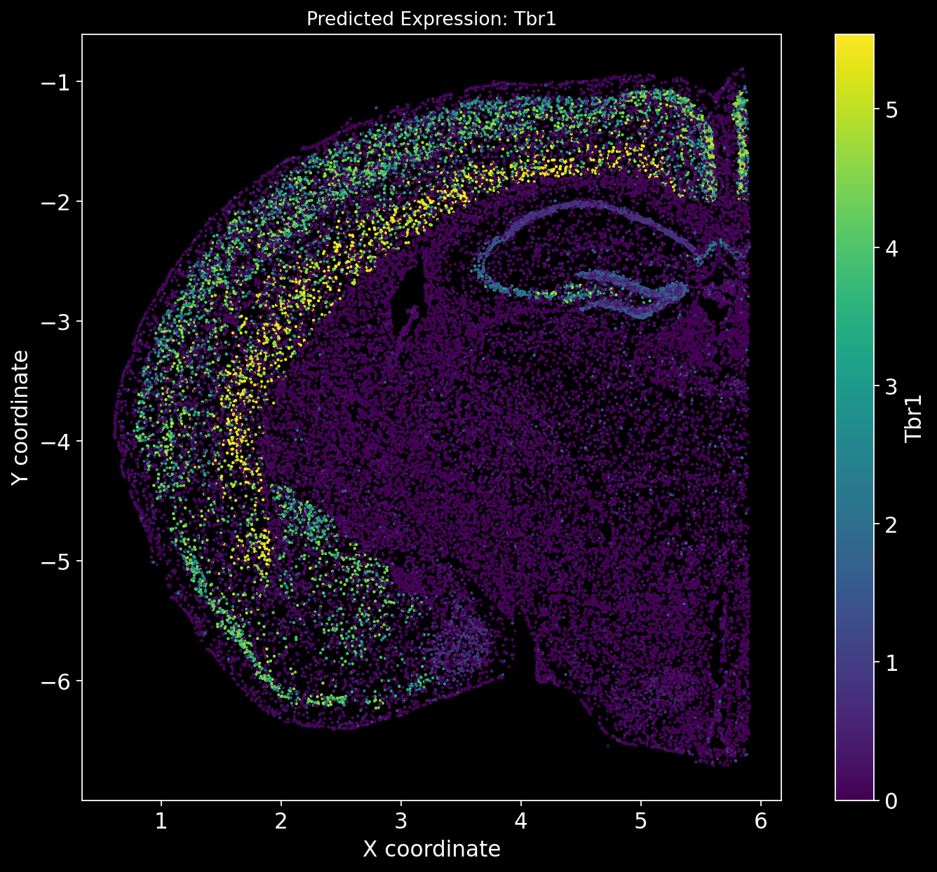
There is no definitive ground truth for the real gene expression profiles of these genes. However, an alternative approach could be to plot region-specific genes and verify whether their expression aligns with the expected brain regions.
For example, Tbr1 is known to be Isocortex-specific; does its expression show higher levels in the Isocortex? Similarly, Foxp2 is Striatum-specific; does it exhibit a Striatum-specific expression pattern?
Use this resource to check region-specific gene expression.
Is there any other gene expression (NOT measured in the spatial dataset) you would like to predict?
Can you think of other genes that we could use to visually validate the accuracy of SpaGE by checking if their expression patterns correspond to their known brain regions? Plot them!
#Gene_set = [...]

#predict_unmeasured_genes(Gene_set)
# Record the end time
end_time = time.time()
# Calculate elapsed time in minutes
elapsed_time = (end_time - start_time) / 60
print(f"Execution Time SpaGE: {elapsed_time:.2f} minutes")Execution Time SpaGE: 12.48 minutesUnmeasured gene imputation with Tangram
start_time = time.time()import scanpy as sc
import tangram as tg
import seaborn as sns
import pandas as pd
import matplotlib.pyplot as plt
from sklearn.preprocessing import MinMaxScaler
sc.settings.verbosity = 3
sc.settings.set_figure_params(dpi=80, facecolor="white")genes_keep = markers+['Clcc1', 'Timp4', 'Ankzf1', 'Hyal4']
adata_sc = adata_sc[:,adata_sc.var.index.isin(genes_keep)]len(genes_keep)Common gene set between reference and spatial dataset
We want to select our training genes. These genes are shared between the two datasets and should capture the biological variance between cell types. For this, we first compute marker genes on the single-cell data and then use Tangram’s preprocessing function to subset to those genes that are also present in the spatial data.
markers = list(set.intersection(set(adata_sc.var_names), set(adata_section.var_names)))
len(markers)
tg.pp_adatas does the following:
Computes the overlap between single-cell data and spatial data on the list of genes provided in the genes argument Stores the resulting gene set under ‘training_genes’ in both adata objects under the .uns key Enforces consistent ordering of the genes To reduce potential naming errors gene names are converted to lower case. To prevent this behaviour set gene_to_lowercase = False.
tg.pp_adatas(adata_sc, adata_section, genes=markers)Let us check that the function performs as we expect:
assert "training_genes" in adata_sc.uns
assert "training_genes" in adata_section.uns

print(f"Number of training_genes: {len(adata_sc.uns['training_genes'])}")#markersComputing the map from single-cells to spatial voxels
Having specified the training genes, we can now create the map from dissociated single-cell measurements to the spatial locations. For this, we are going to use the map_cells_to_space function from tangram. This function has two different modes, mode=‘cells’ and mode=‘clusters’. The latter only maps averaged single-cells which makes the mapping computationally faster and more robust when mapping between specimen. However, as we are interested in imputing our spatial data, we will rely on the cell mode which might require access to a GPU for reasonable runtime.
ad_map = tg.map_cells_to_space(
    adata_sc,
    adata_section,
    mode="cells",
    density_prior="rna_count_based",
    num_epochs=500,
    device="cpu",  # or: cpu
)
The resulting ad_map is itself an AnnData object. Let us inspect it:
ad_mapWe observe that Tangram’s mapping from cell i to spatial voxels j is stored in the .X property of ad_map.
Hence, the meaning of the .var and .obs also changes:
in .var we have the available metadata of the spatial data, adata_st in .obs we have the available metadata of the single-cell data, adata_sc In addition, the information about the training run is stored in the .uns key, see .uns[‘training_genes_df’] and .uns[training_history].
Now, we can project the genes present in the single-cell data to the spatial locations. This is easily achieved by multiplying the mapping matrix stored in ad_map with the original single-cell data stored in adata_sc. Tangram already provides a convenience function which takes in a mapping and the corresponding single-cell data. The result is a spatial voxel by genes matrix which technically is identical to the original spatial data adata_st but contains expression values for all genes.
ad_ge = tg.project_genes(adata_map=ad_map, adata_sc=adata_sc)
ad_ge
Next, we will compare the new spatial data with the original measurements. This will provide us with a better feeling why some training scores might be bad. Note that this explicit mapping of Tangram relies on entirely different premises than those in probabilistic models. Here, we are inclined to trust the predicted gene expression patterns based on the good mapping performance of most training genes. The fact the some genes show a very sparse and dispersed spatial signal can be understood a result of technical dropout of the spatial technology rather than a shortcoming of the mapping method.
genes = ["tek", "stab2", "hc"]
ad_map.uns["train_genes_df"].loc[genes]
# The comparison between original measurements on predicted ones is easily done with tangram
tg.plot_genes_sc(
genes,
adata_measured=adata_st[adata_st.obs.FOV == 0],
adata_predicted=ad_ge[ad_ge.obs.FOV == 0],
perc=0.02,
spot_size=50,
)Plotting genes that were not part of the training data
We can also inspect genes there were part of the training genes but not detected in the spatial data.
genes = ["rp1", "sox17", "mrpl15"]
tg.plot_genes_sc(
    genes,
    adata_measured=adata_st[adata_st.obs.FOV == 0],
    adata_predicted=ad_ge[ad_ge.obs.FOV == 0],
    perc=0.02,
    spot_size=50,
)
# Code to be executed
# ... Your code here ...

# Record the end time
end_time = time.time()

# Calculate elapsed time in minutes
elapsed_time = (end_time - start_time) / 60
print(f"Execution Time Tangram: {elapsed_time:.2f} minutes")
Spatial omics data are clustered to define both cell types and tissue domains. BANKSY is an algorithm that unifies these two spatial clustering problems by embedding cells in a product space of their own and the local neighborhood transcriptome, representing cell state and microenvironment, respectively.

This is done by augmenting the original gene-cell expression matrix (purple) with neighborhood-averaged expression matrices corresponding to the mean local expression (dark pink) and the AGF (light pink). Here, λ is a mixing parameter that controls the importance of cells’ own expression and neighborhood expression effects, G(r) is a radially symmetric Gaussian kernel that decays from magnitude 1 at distance = 0.
start_time = time.time()from banksy_utils.load_data import load_adata, display_adata
from banksy_utils.filter_utils import normalize_total, filter_hvg, print_max_min
# Normalizes the AnnData object
adata_section = normalize_total(adata_section)--- Max-Min before normalization -----
Displaying max and min of Dataset
Max: 368.0, Min: 0.0
--- Max-Min after normalization -----
Displaying max and min of Dataset
Max: 256.98077392578125, Min: 0.0
Generate spatial weights graph
In BANKSY, we imagine edges / connections in the graph to represent neighbour relationships between cells
BANKSY requires the following specifications in the main BANKSY algorithm:
1. The number of spatial neighbours num_neighbours (k_geom) parameter.
2. Assigning weights (dependent on inter-cell spatial distances) to edges in the connected spatial graph. By default, we use the gaussian decay option, where weights decay as a function of distance to the index cell with \(\sigma\) = sigma.
3. The Azumithal Gabor Filter parameter max_m which indicates whether to use the AGF (max_m = 1) or just the mean expression (max_m = 0). By default, we set max_m = 1.
Construction of the spatial \(k_{geom}\) Nearest-Neighbour graph
We represent connections between cells and its neighbours in a graph \(G = \{N,E,W\}\), comprising of a set of nodes \(n \in N\). Edges represent connectivity between cells \(e \in E\), the edges are weighted \(w \in W\) as a function of the spatial distance between cells.
from banksy.main import median_dist_to_nearest_neighbour

coord_keys = ('x', 'y', 'X_spatial')

# set parameters
plot_graph_weights = True
k_geom = 15 # number of neighbors
max_m = 1 # azumithal transform up to kth order
nbr_weight_decay = "scaled_gaussian" # can also be "reciprocal", "uniform" or "ranked"

# Find median distance to closest neighbours, the median distance will be `sigma`
nbrs = median_dist_to_nearest_neighbour(adata_section, key = coord_keys[2])
Median distance to closest cell = 0.011451999258720952

---- Ran median_dist_to_nearest_neighbour in 0.10 s ----
Generate spatial weights from distance
Here, we generate the spatial weights using the gaussian decay function from the median distance to the k-th nearest neighbours as specified earlier.
from banksy.initialize_banksy import initialize_banksy

plt.style.use('default')

banksy_dict = initialize_banksy(
    adata_section,
    coord_keys,
    k_geom,
    nbr_weight_decay=nbr_weight_decay,
    max_m=max_m,
    plt_edge_hist=False,
    plt_nbr_weights=True,
    plt_agf_angles=False, # takes long time to plot
    plt_theta=False,
)
Median distance to closest cell = 0.011451999258720952

---- Ran median_dist_to_nearest_neighbour in 0.10 s ----

---- Ran generate_spatial_distance_graph in 0.22 s ----

---- Ran row_normalize in 0.14 s ----

---- Ran generate_spatial_weights_fixed_nbrs in 1.53 s ----

----- Plotting Edge Histograms for m = 0 -----

Edge weights (distances between cells): median = 0.03694992316725689, mode = 0.03778937001055409

---- Ran plot_edge_histogram in 0.08 s ----


Edge weights (weights between cells): median = 0.05769858243908976, mode = 0.03646096900941189

---- Ran plot_edge_histogram in 0.08 s ----

---- Ran generate_spatial_distance_graph in 0.32 s ----

---- Ran theta_from_spatial_graph in 0.43 s ----

---- Ran row_normalize in 0.14 s ----

---- Ran generate_spatial_weights_fixed_nbrs in 2.19 s ----

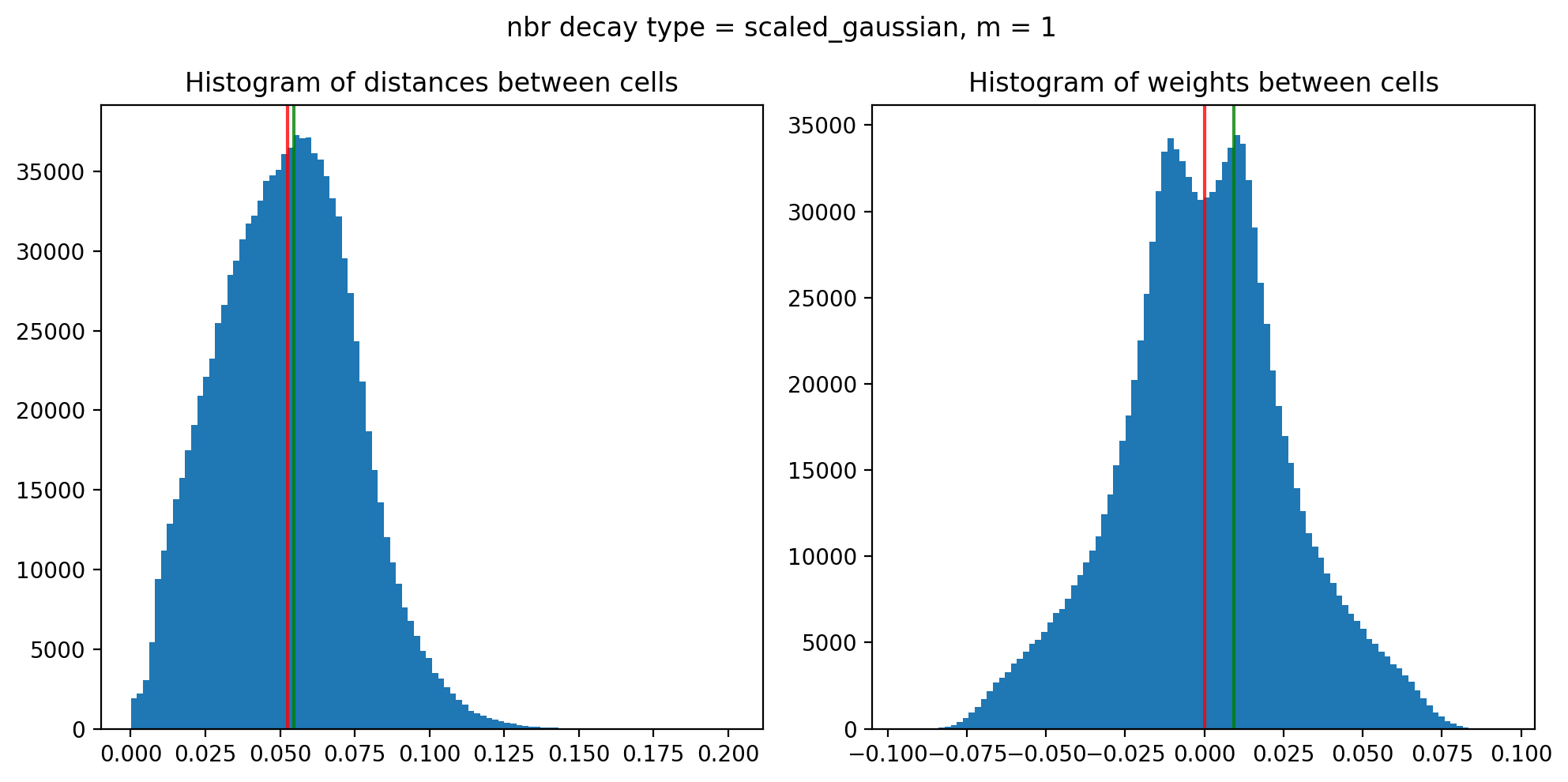
----- Plotting Edge Histograms for m = 1 -----

Edge weights (distances between cells): median = 0.05241795688794886, mode = 0.054503027119080505

---- Ran plot_edge_histogram in 0.10 s ----


Edge weights (weights between cells): median = (6.059505504588136e-05-0.009422017917133459j), mode = 0.009314181436698696

---- Ran plot_edge_histogram in 0.16 s ----

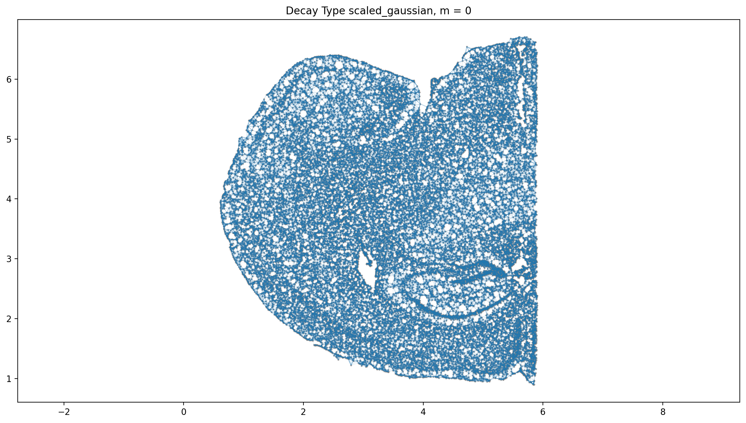
----- Plotting Weights Graph -----
Maximum weight: 0.22787938934483182

---- Ran plot_graph_weights in 5.46 s ----

Maximum weight: (0.09488573219546165+0.01411718561667858j)

---- Ran plot_graph_weights in 11.06 s ----

----- Plotting theta Graph -----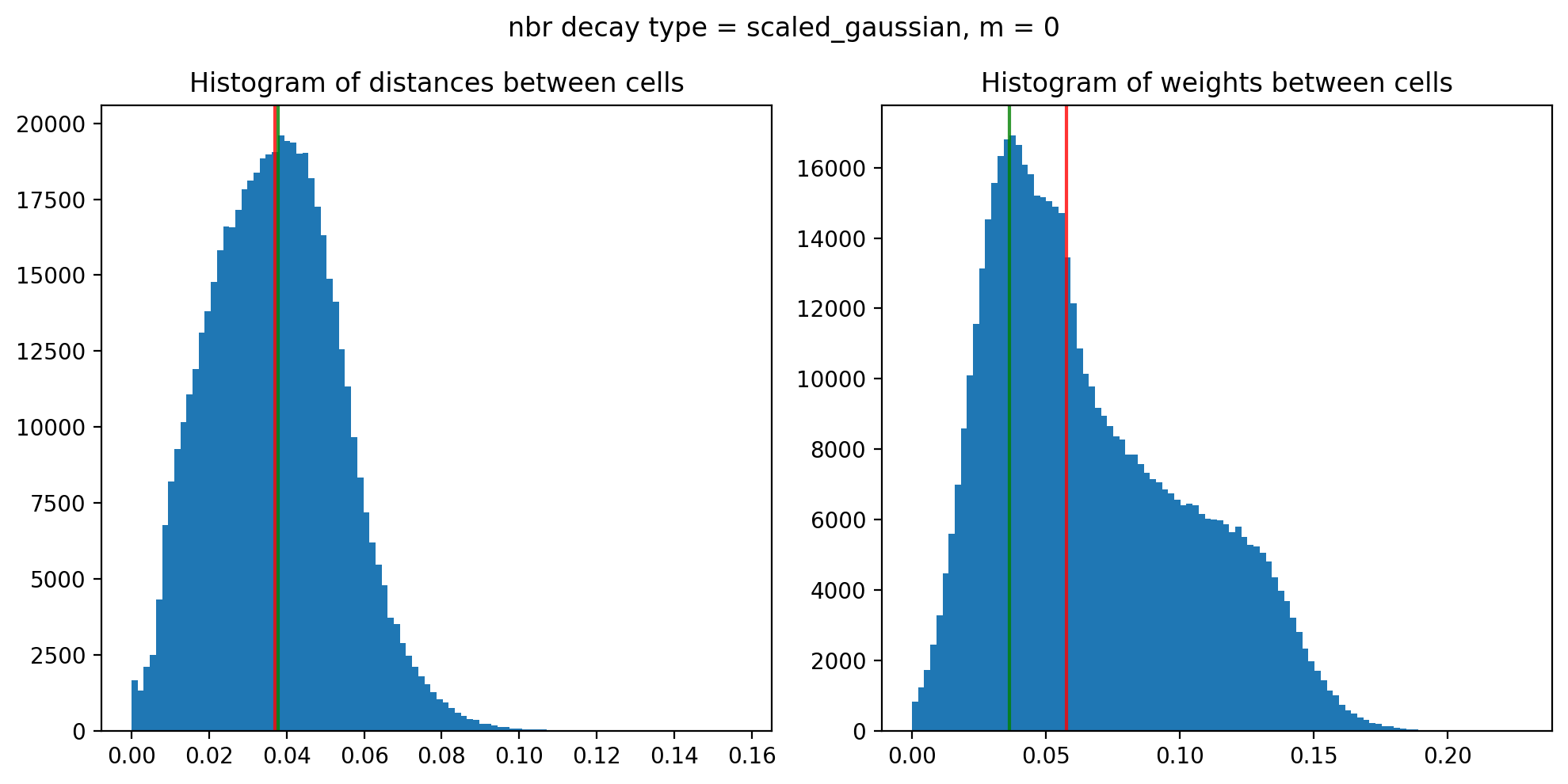
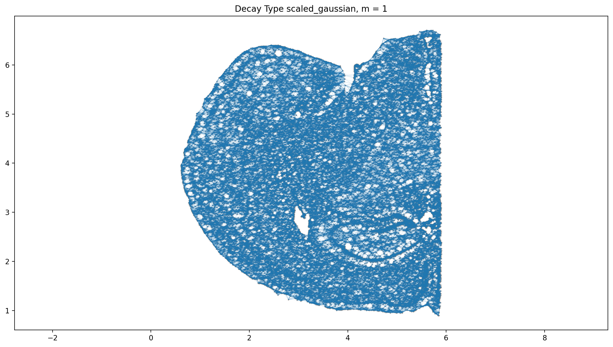
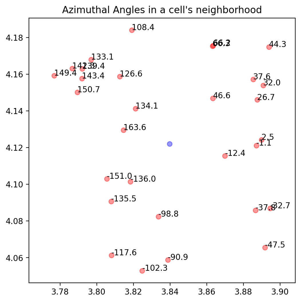
Generate BANKSY matrix
λ is a mixing parameter that controls the importance of cells’ own expression and neighborhood expression effects, it takes values from 0, being spatial information not used in the clustering, to 1, giving the maximum importance to the neighborhood expression.
To generate the BANKSY matrix, we proceed with the following:
1. Matrix multiply sparse CSR weights matrix with cell-gene matrix to get neighbour matrix and the AGF matrix if max_m > 1
2. Z-score both matrices along genes
3. Multiply each matrix by a weighting factor \(\lambda\) (We refer to this parameter as lambda in our manuscript and code)
4. Concatenate the matrices along the genes dimension in the form -> horizontal_concat(cell_mat, nbr_mat, agf_mat)
Here, we save all the results in the dictionary (banksy_dict), which contains the results from the subsequent operations for BANKSY.
from banksy.embed_banksy import generate_banksy_matrix

# The following are the main hyperparameters for BANKSY
resolutions = [0.1] # clustering resolution for UMAP
pca_dims = [20] # Dimensionality in which PCA reduces to
lambda_list = [0.5,0.75] # list of lambda parameters

banksy_dict, banksy_matrix = generate_banksy_matrix(adata_section, banksy_dict, lambda_list, max_m)
Runtime Oct-25-2024-13-18
1122 genes to be analysed:
Gene List:
Index(['Htr7', 'Gzmk', 'Arhgap36', 'Sema3c', 'Rxrg', 'Itga8', 'Glp2r', 'Ramp3',
'Car12', 'Chn2',
...
'Galnt14', 'Kcnh8', 'Pifo', 'Epb41l4a', 'Matn2', 'Gata3', 'Fat1',
'Zim1', 'Lmo1', 'Cntnap3'],
dtype='object', name='gene_symbol', length=1122)
Decay Type: scaled_gaussian
Weights Object: {'weights': {0: <Compressed Sparse Row sparse matrix of dtype 'float64'
with 556020 stored elements and shape (37068, 37068)>, 1: <Compressed Sparse Row sparse matrix of dtype 'complex128'
with 1112040 stored elements and shape (37068, 37068)>}}
Nbr matrix | Mean: 0.29 | Std: 1.06
Size of Nbr | Shape: (37068, 1122)
Top 3 entries of Nbr Mat:
[[0.7558483 0. 0.04643741]
[0.47232749 0. 0. ]
[0.58894371 0. 0. ]]
AGF matrix | Mean: 0.11 | Std: 0.3
Size of AGF mat (m = 1) | Shape: (37068, 1122)
Top entries of AGF:
[[0.06324971 0. 0.02116232]
[0.06511702 0. 0. ]
[0.17339295 0. 0. ]]
Ran 'Create BANKSY Matrix' in 0.16 mins
Cell by gene matrix has shape (37068, 1122)
Scale factors squared: [0.5 0.33333333 0.16666667]
Scale factors: [0.70710678 0.57735027 0.40824829]
Shape of BANKSY matrix: (37068, 3366)
Type of banksy_matrix: <class 'anndata._core.anndata.AnnData'>
Scale factors squared: [0.25 0.5 0.25]
Scale factors: [0.5 0.70710678 0.5 ]
Shape of BANKSY matrix: (37068, 3366)
Type of banksy_matrix: <class 'anndata._core.anndata.AnnData'>
Append Non-spatial results to the banksy_dict for comparsion
from banksy.main import concatenate_all

banksy_dict["nonspatial"] = {
    # Here we simply append the nonspatial matrix (adata.X) to obtain the nonspatial clustering results
    0.0: {"adata": concatenate_all([adata_section.X], 0, adata=adata_section), }
}

print(banksy_dict['nonspatial'][0.0]['adata'])
Scale factors squared: [1.]
Scale factors: [1.]
AnnData object with n_obs × n_vars = 37068 × 1122
obs: 'brain_section_label', 'feature_matrix_label', 'donor_label', 'donor_genotype', 'donor_sex', 'cluster_alias', 'x', 'y', 'z', 'subclass_confidence_score', 'cluster_confidence_score', 'high_quality_transfer', 'neurotransmitter', 'class', 'subclass', 'supertype', 'cluster', 'neurotransmitter_color', 'class_color', 'subclass_color', 'supertype_color', 'cluster_color'
var: 'gene_identifier', 'name', 'mapped_ncbi_identifier', 'is_nbr', 'k'Reduce dimensions of each data matrix
We utilize two common methods for dimensionality reduction:
1. PCA (using scikit-learn), we reduce the size of the matrix from \(3*N_{genes}\) to pca_dims. As a default settings, we reduce to 20 dimensions.
2. UMAP (UMAP package), which we use to visualize expressions of clusters in the umap space (2-D space).
from banksy_utils.umap_pca import pca_umap

pca_umap(banksy_dict,
         pca_dims = pca_dims,
         add_umap = True,
         plt_remaining_var = False,
         )
Current decay types: ['scaled_gaussian', 'nonspatial']
Reducing dims of dataset in (Index = scaled_gaussian, lambda = 0.5)
==================================================
Setting the total number of PC = 20
Original shape of matrix: (37068, 3366)
Reduced shape of matrix: (37068, 20)
------------------------------------------------------------
min_value = -19.044376046754554, mean = 3.8829508173479005e-15, max = 25.000292889223665
Conducting UMAP and adding embeddings to adata.obsm["reduced_pc_20_umap"]
UMAP embedding
------------------------------------------------------------
shape: (37068, 2)
AxisArrays with keys: reduced_pc_20, reduced_pc_20_umap
Reducing dims of dataset in (Index = scaled_gaussian, lambda = 0.75)
==================================================
Setting the total number of PC = 20
Original shape of matrix: (37068, 3366)
Reduced shape of matrix: (37068, 20)
------------------------------------------------------------
min_value = -23.531916398264165, mean = 7.53250440930962e-16, max = 26.9273923955795
Conducting UMAP and adding embeddings to adata.obsm["reduced_pc_20_umap"]
UMAP embedding
------------------------------------------------------------
shape: (37068, 2)
AxisArrays with keys: reduced_pc_20, reduced_pc_20_umap
Reducing dims of dataset in (Index = nonspatial, lambda = 0.0)
==================================================
Setting the total number of PC = 20
Original shape of matrix: (37068, 1122)
Reduced shape of matrix: (37068, 20)
------------------------------------------------------------
min_value = -18.594362258911133, mean = -5.210476388128882e-07, max = 30.442607879638672
Conducting UMAP and adding embeddings to adata.obsm["reduced_pc_20_umap"]
UMAP embedding
------------------------------------------------------------
shape: (37068, 2)
AxisArrays with keys: reduced_pc_20, reduced_pc_20_umapCluster cells using a partition algorithm
We then cluster cells using the leiden algorithm partition methods. Other clustering algorithms include louvain (another resolution based clustering algorithm), or mclust (a clustering based on gaussian mixture model).
from banksy.cluster_methods import run_Leiden_partition
seed = 0
results_df, max_num_labels = run_Leiden_partition(
    banksy_dict,
    resolutions,
    num_nn = 50,
    num_iterations = -1,
    partition_seed = seed,
    match_labels = True,
)
Decay type: scaled_gaussian
Neighbourhood Contribution (Lambda Parameter): 0.5
reduced_pc_20
reduced_pc_20_umap
PCA dims to analyse: [20]
====================================================================================================
Setting up partitioner for (nbr decay = scaled_gaussian), Neighbourhood contribution = 0.5, PCA dimensions = 20)
====================================================================================================
Nearest-neighbour weighted graph (dtype: float64, shape: (37068, 37068)) has 1853400 nonzero entries.
---- Ran find_nn in 17.81 s ----
Nearest-neighbour connectivity graph (dtype: int16, shape: (37068, 37068)) has 1853400 nonzero entries.
(after computing shared NN)
Allowing nearest neighbours only reduced the number of shared NN from 16755666 to 1852311.
Shared nearest-neighbour (connections only) graph (dtype: int16, shape: (37068, 37068)) has 1826005 nonzero entries.
Shared nearest-neighbour (number of shared neighbours as weights) graph (dtype: int16, shape: (37068, 37068)) has 1826005 nonzero entries.
sNN graph data:
[17 38 36 ... 11 7 10]
---- Ran shared_nn in 1.41 s ----
-- Multiplying sNN connectivity by weights --
shared NN with distance-based weights graph (dtype: float64, shape: (37068, 37068)) has 1826005 nonzero entries.
shared NN weighted graph data: [0.19430965 0.19593433 0.19699834 ... 0.19985507 0.21744874 0.2667582 ]
Converting graph (dtype: float64, shape: (37068, 37068)) has 1826005 nonzero entries.
---- Ran csr_to_igraph in 0.49 s ----
Resolution: 0.1
------------------------------
---- Partitioned BANKSY graph ----
modularity: 0.85
14 unique labels:
[ 0 1 2 3 4 5 6 7 8 9 10 11 12 13]
---- Ran partition in 3.19 s ----
No annotated labels
Neighbourhood Contribution (Lambda Parameter): 0.75
reduced_pc_20
reduced_pc_20_umap
PCA dims to analyse: [20]
====================================================================================================
Setting up partitioner for (nbr decay = scaled_gaussian), Neighbourhood contribution = 0.75, PCA dimensions = 20)
====================================================================================================
Nearest-neighbour weighted graph (dtype: float64, shape: (37068, 37068)) has 1853400 nonzero entries.
---- Ran find_nn in 14.13 s ----
Nearest-neighbour connectivity graph (dtype: int16, shape: (37068, 37068)) has 1853400 nonzero entries.
(after computing shared NN)
Allowing nearest neighbours only reduced the number of shared NN from 18134622 to 1852781.
Shared nearest-neighbour (connections only) graph (dtype: int16, shape: (37068, 37068)) has 1829094 nonzero entries.
Shared nearest-neighbour (number of shared neighbours as weights) graph (dtype: int16, shape: (37068, 37068)) has 1829094 nonzero entries.
sNN graph data:
[20 36 36 ... 15 8 6]
---- Ran shared_nn in 1.46 s ----
-- Multiplying sNN connectivity by weights --
shared NN with distance-based weights graph (dtype: float64, shape: (37068, 37068)) has 1829094 nonzero entries.
shared NN weighted graph data: [0.15680677 0.15687761 0.15754264 ... 0.30728138 0.31398833 0.5863947 ]
Converting graph (dtype: float64, shape: (37068, 37068)) has 1829094 nonzero entries.
---- Ran csr_to_igraph in 0.51 s ----
Resolution: 0.1
------------------------------
---- Partitioned BANKSY graph ----
modularity: 0.83
11 unique labels:
[ 0 1 2 3 4 5 6 7 8 9 10]
---- Ran partition in 4.83 s ----
No annotated labels
Decay type: nonspatial
Neighbourhood Contribution (Lambda Parameter): 0.0
reduced_pc_20
reduced_pc_20_umap
PCA dims to analyse: [20]
====================================================================================================
Setting up partitioner for (nbr decay = nonspatial), Neighbourhood contribution = 0.0, PCA dimensions = 20)
====================================================================================================
Nearest-neighbour weighted graph (dtype: float64, shape: (37068, 37068)) has 1853400 nonzero entries.
---- Ran find_nn in 18.57 s ----
Nearest-neighbour connectivity graph (dtype: int16, shape: (37068, 37068)) has 1853400 nonzero entries.
(after computing shared NN)
Allowing nearest neighbours only reduced the number of shared NN from 27067154 to 1851869.
Shared nearest-neighbour (connections only) graph (dtype: int16, shape: (37068, 37068)) has 1803981 nonzero entries.
Shared nearest-neighbour (number of shared neighbours as weights) graph (dtype: int16, shape: (37068, 37068)) has 1803981 nonzero entries.
sNN graph data:
[22 7 27 ... 19 19 6]
---- Ran shared_nn in 1.70 s ----
-- Multiplying sNN connectivity by weights --
shared NN with distance-based weights graph (dtype: float64, shape: (37068, 37068)) has 1803981 nonzero entries.
shared NN weighted graph data: [0.18722369 0.1876801 0.18798157 ... 0.18788907 0.19163482 0.22798553]
Converting graph (dtype: float64, shape: (37068, 37068)) has 1803981 nonzero entries.
---- Ran csr_to_igraph in 0.46 s ----
Resolution: 0.1
------------------------------
---- Partitioned BANKSY graph ----
modularity: 0.89
17 unique labels:
[ 0 1 2 3 4 5 6 7 8 9 10 11 12 13 14 15 16]
---- Ran partition in 3.08 s ----
No annotated labels
After sorting Dataframe
Shape of dataframe: (3, 7)
Maximum number of labels = 17
Indices of sorted list: [2 1 0]
Expanding labels with ids: [ 0 1 2 3 4 5 6 7 8 9 10] so that ids range from 0 to 16
Label ids zerod: [ 0 1 2 3 4 5 6 7 8 9 10].
0 to be inserted between each id: [0 0 0 0 0 0 0 0 0 0 0]
6 extra rows to be randomly inserted: [1 1 0 0 0 1 0 1 1 1]
New ids: [ 0 2 4 5 6 7 9 10 12 14 16]
---- Ran expand_labels in 0.00 s ----
---- Ran match_labels in 0.00 s ----
---- Ran match_labels in 0.00 s ----
Matched Labels| decay | lambda_param | num_pcs | resolution | num_labels | labels | adata | relabeled | |
|---|---|---|---|---|---|---|---|---|
| nonspatial_pc20_nc0.00_r0.10 | nonspatial | 0.00 | 20 | 0.1 | 17 | Label object:\nNumber of labels: 17, number of... | [[[View of AnnData object with n_obs × n_vars ... | Label object:\nNumber of labels: 17, number of... |
| scaled_gaussian_pc20_nc0.50_r0.10 | scaled_gaussian | 0.50 | 20 | 0.1 | 14 | Label object:\nNumber of labels: 14, number of... | [[[View of AnnData object with n_obs × n_vars ... | Label object:\nNumber of labels: 14, number of... |
| scaled_gaussian_pc20_nc0.75_r0.10 | scaled_gaussian | 0.75 | 20 | 0.1 | 11 | Label object:\nNumber of labels: 11, number of... | [[[View of AnnData object with n_obs × n_vars ... | Label object:\nNumber of labels: 11, number of... |
Plot results
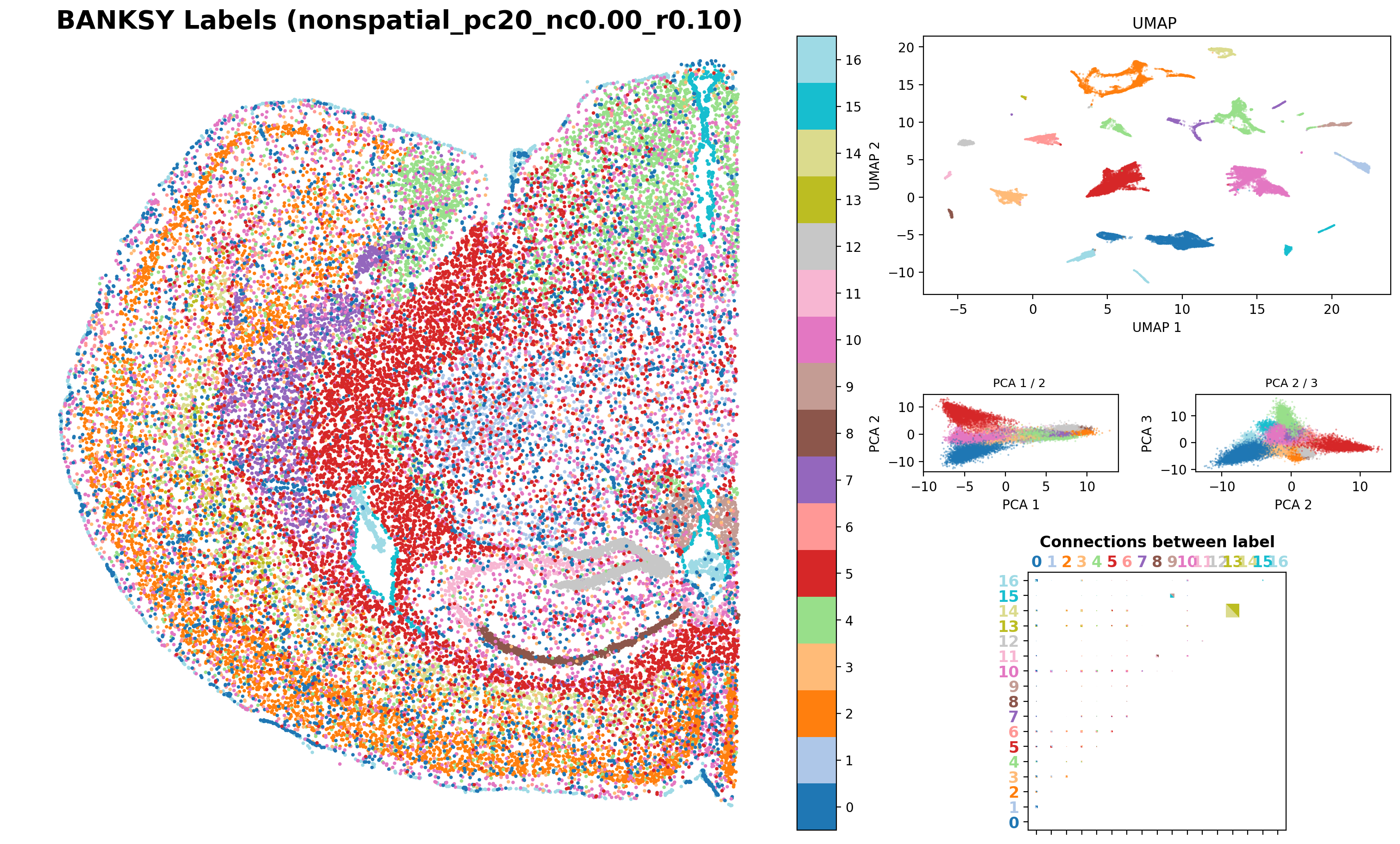
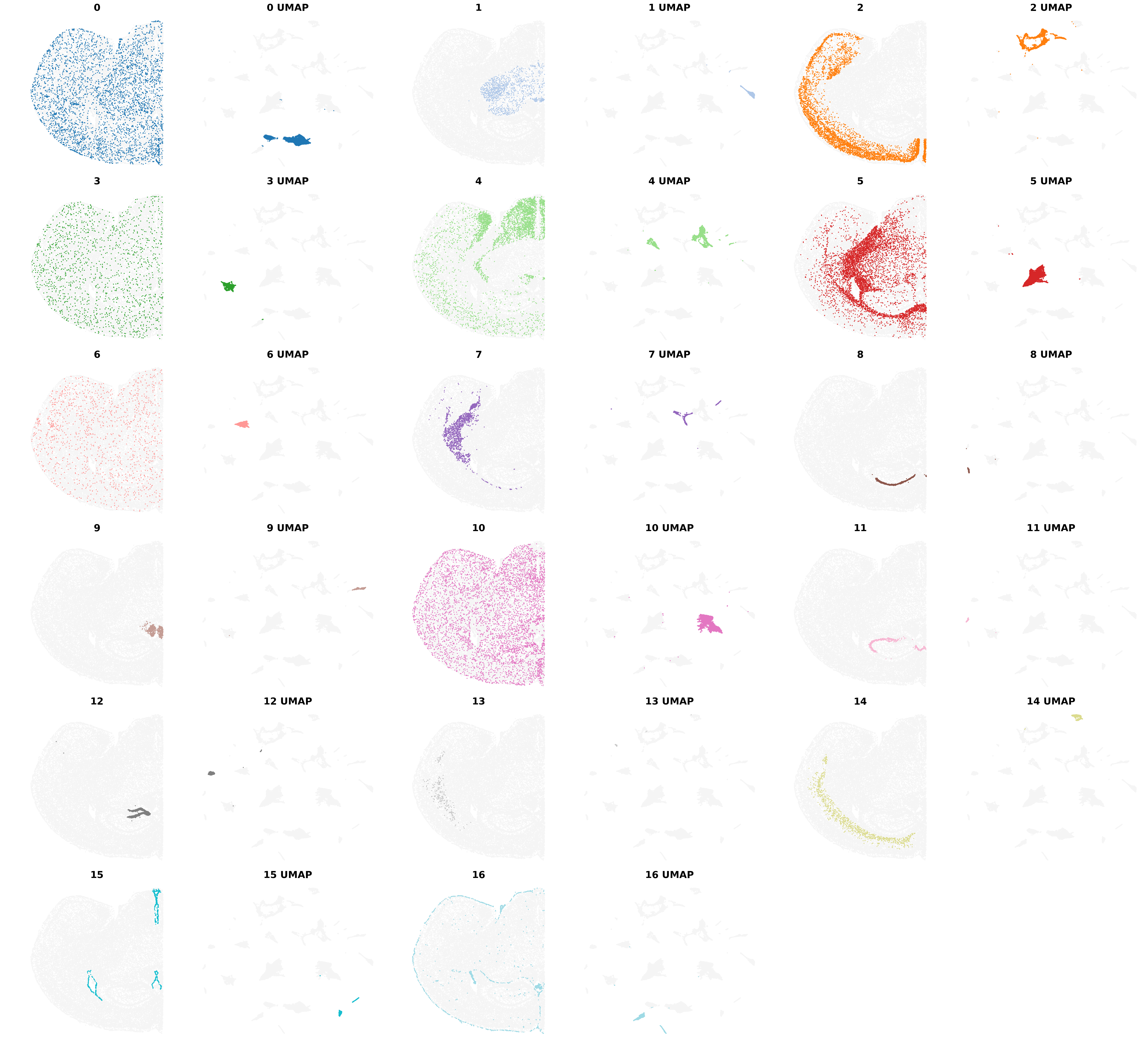
Visualize the clustering results from BANKSY, including the clusters from the Umap embbedings
from banksy.plot_banksy import plot_results

c_map =  'tab20' # specify color map
weights_graph =  banksy_dict['scaled_gaussian']['weights'][0]

file_path = '/exports/humgen/bmanzato/spatial_workshop/banksy_output/'

plot_results(
    results_df,
    weights_graph,
    c_map,
    match_labels = True,
    coord_keys = coord_keys,
    max_num_labels  =  max_num_labels,
    save_path = os.path.join(file_path, 'tmp_png'),
    save_fig = True, # save the spatial map of all clusters
    save_seperate_fig = True, # save the figure of all clusters plotted seperately
)
Saving figure at /exports/humgen/bmanzato/spatial_workshop/banksy_output/tmp_png/slideseq_mousecerebellum_nonspatial_pc20_nc0.00_r0.10_spatialmap.png
number of labels: 17
---- Ran plot_2d_embeddings in 0.00 s ----
number of labels: 17
---- Ran plot_2d_embeddings in 0.01 s ----
number of labels: 17
---- Ran plot_2d_embeddings in 0.00 s ----
---- Ran row_normalize in 0.00 s ----
matrix multiplying labels x weights x labels-transpose ((17, 37068) x (37068, 37068) x (37068, 17))
Saving figure at /exports/humgen/bmanzato/spatial_workshop/banksy_output/tmp_png/slideseq_mousecerebellum_scaled_gaussian_pc20_nc0.50_r0.10_spatialmap.png
number of labels: 14
---- Ran plot_2d_embeddings in 0.01 s ----
number of labels: 14
---- Ran plot_2d_embeddings in 0.01 s ----
number of labels: 14
---- Ran plot_2d_embeddings in 0.00 s ----
---- Ran row_normalize in 0.00 s ----
matrix multiplying labels x weights x labels-transpose ((14, 37068) x (37068, 37068) x (37068, 14))
Saving figure at /exports/humgen/bmanzato/spatial_workshop/banksy_output/tmp_png/slideseq_mousecerebellum_scaled_gaussian_pc20_nc0.75_r0.10_spatialmap.png
number of labels: 11
---- Ran plot_2d_embeddings in 0.00 s ----
number of labels: 11
---- Ran plot_2d_embeddings in 0.01 s ----
number of labels: 11
---- Ran plot_2d_embeddings in 0.00 s ----
---- Ran row_normalize in 0.00 s ----
matrix multiplying labels x weights x labels-transpose ((11, 37068) x (37068, 37068) x (37068, 11))
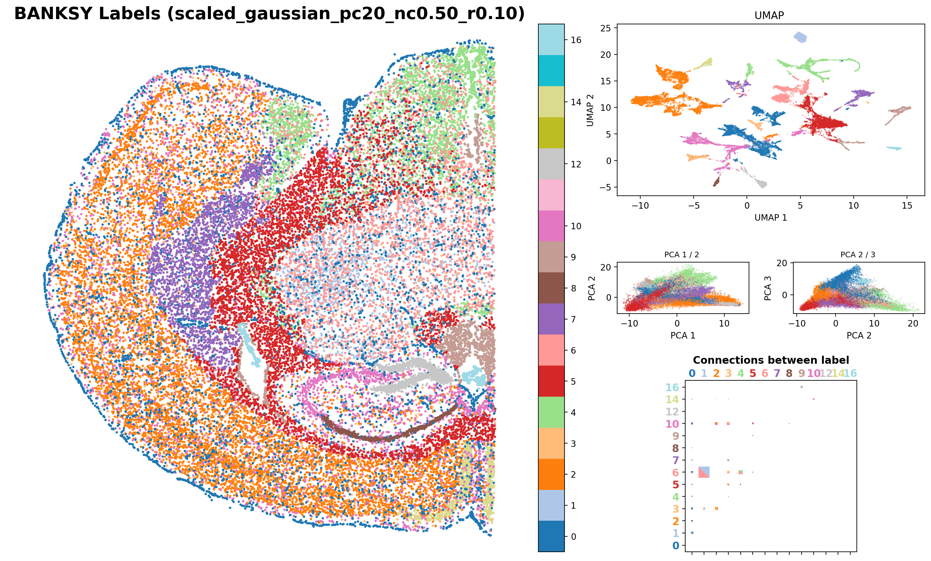
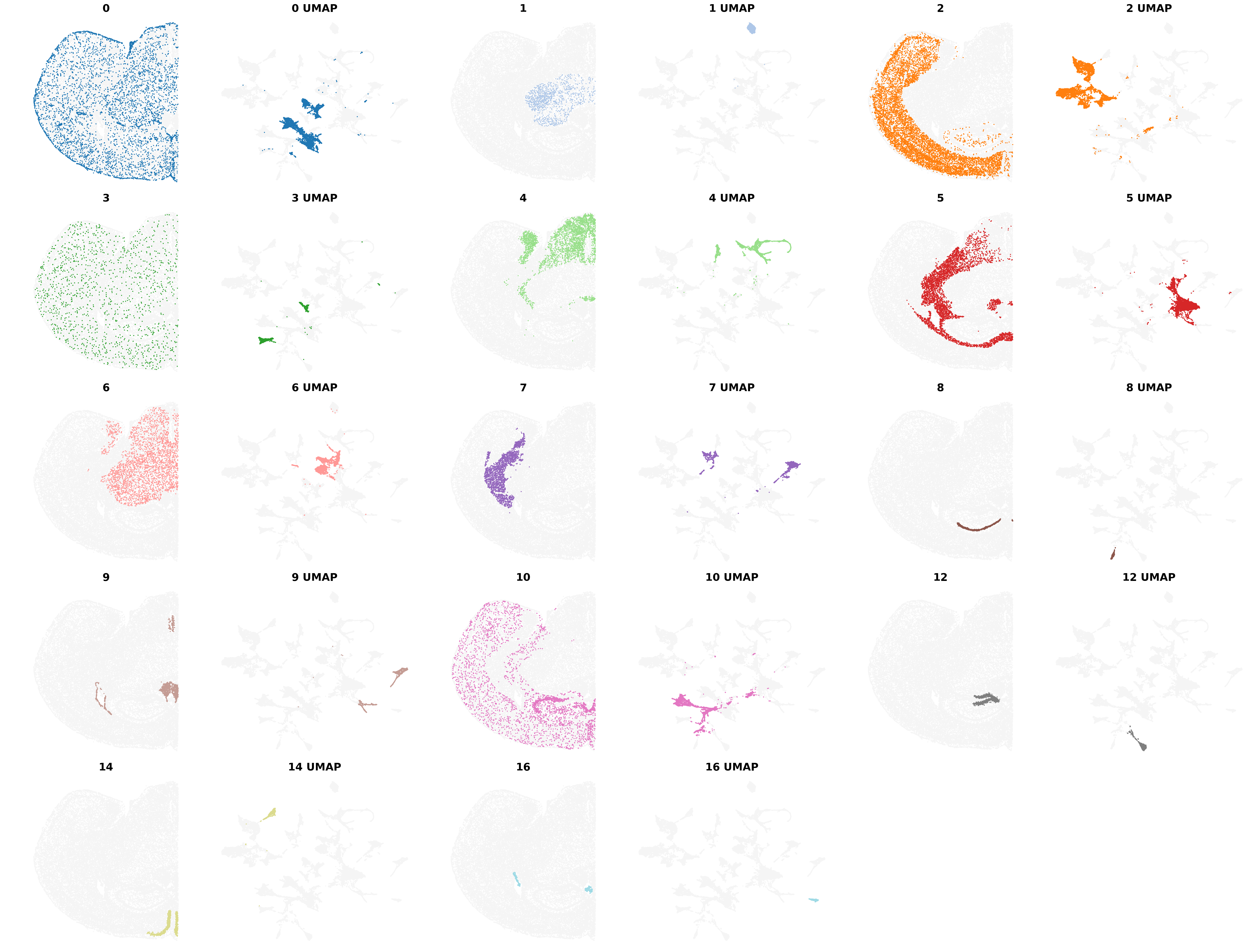
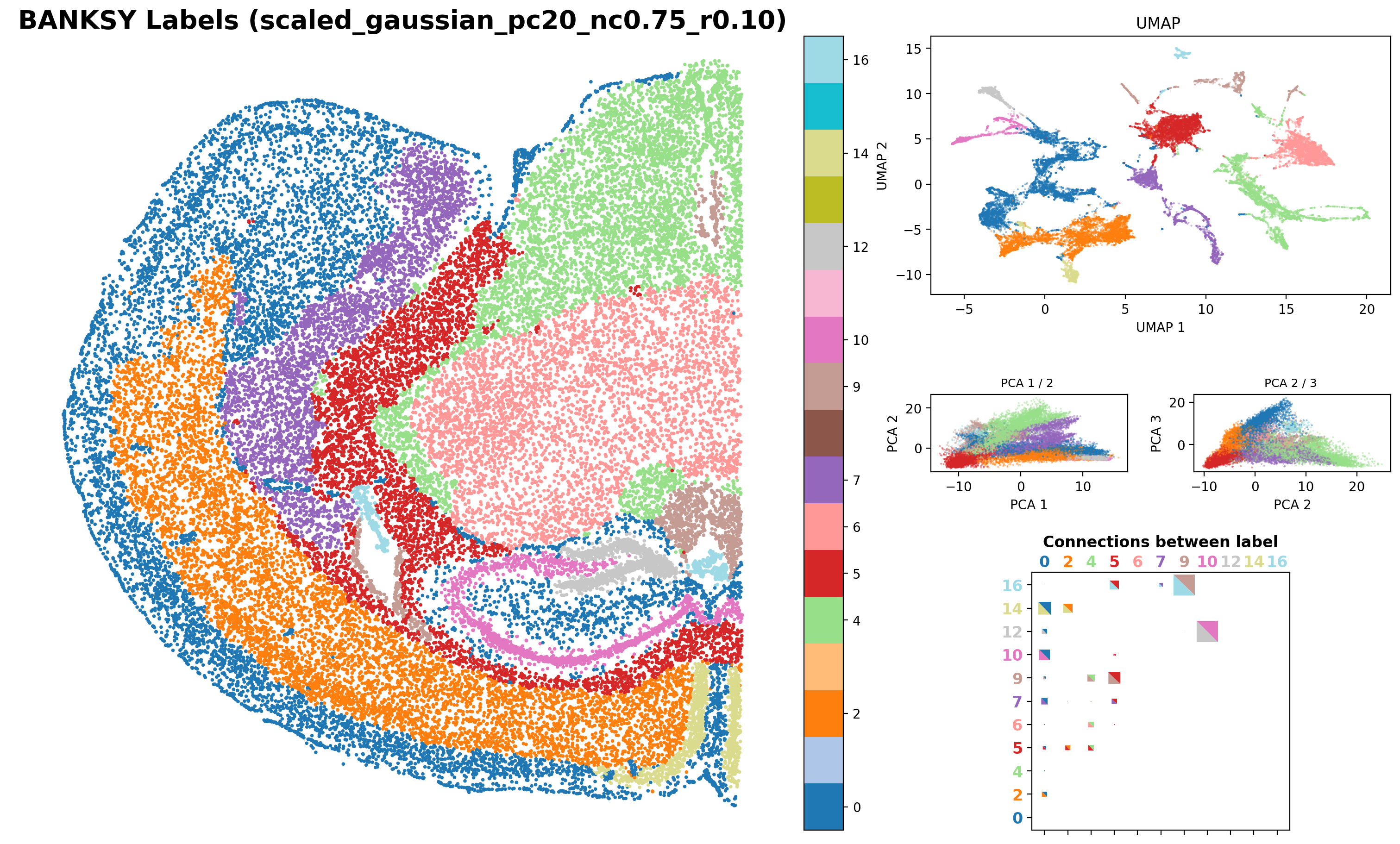
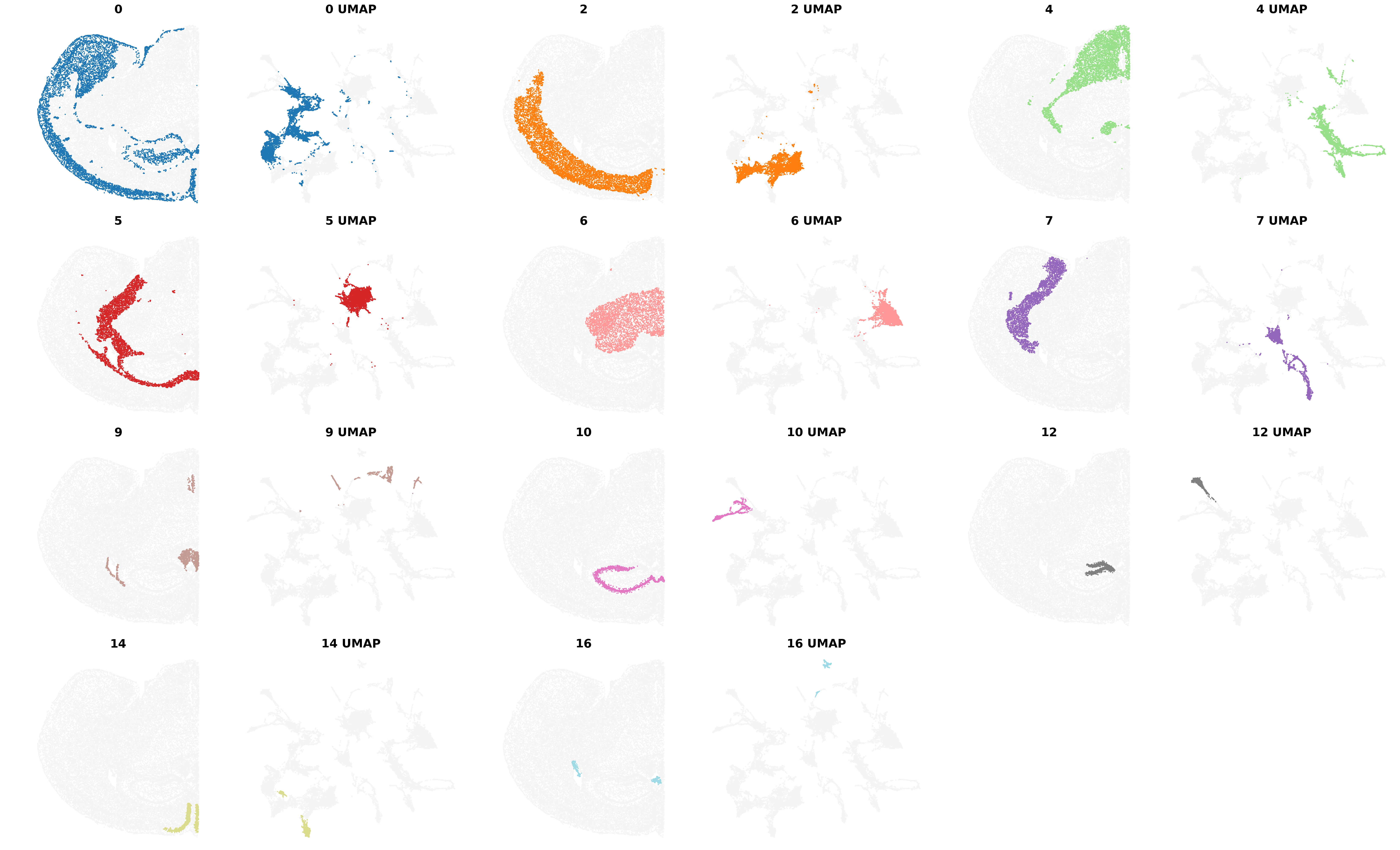
#  Record the end time
end_time = time.time()

# Calculate elapsed time in minutes
elapsed_time = (end_time - start_time) / 60
print(f"Execution Time Banksy: {elapsed_time:.2f} minutes")
Execution Time Banksy: 5.47 minutes What do you expect would happen when we set lambda = 1?
How do you expect the spatial clusters plot to look like?
Re run Banksy changing lambda to 1.
What do you expect would happen when we increase k_geom?
Re run Banksy changing k_geom to 80.
### Investigate Cell Type composition in each Banksy-defined Spatial Domainresults_df_lambda075 = results_df.loc['scaled_gaussian_pc20_nc0.75_r0.10','adata']results_df_lambda075AnnData object with n_obs × n_vars = 37068 × 3366
obs: 'brain_section_label', 'feature_matrix_label', 'donor_label', 'donor_genotype', 'donor_sex', 'cluster_alias', 'x', 'y', 'z', 'subclass_confidence_score', 'cluster_confidence_score', 'high_quality_transfer', 'neurotransmitter', 'class', 'subclass', 'supertype', 'cluster', 'neurotransmitter_color', 'class_color', 'subclass_color', 'supertype_color', 'cluster_color', 'labels_scaled_gaussian_pc20_nc0.75_r0.10'
var: 'gene_identifier', 'name', 'mapped_ncbi_identifier', 'is_nbr', 'k'
obsm: 'reduced_pc_20', 'reduced_pc_20_umap', 'X_spatial'results_df_lambda075.obs['Count'] = 1 # Add a count column if necessary
grouped = results_df_lambda075.obs.groupby(['labels_scaled_gaussian_pc20_nc0.75_r0.10', 'class']).size().reset_index(name='Count')
pivot_df = grouped.pivot_table(index='labels_scaled_gaussian_pc20_nc0.75_r0.10', columns='class', values='Count', aggfunc='sum', fill_value=0)
pivot_df = pivot_df.div(pivot_df.sum(axis=1), axis=0) * 100
fig, ax = plt.subplots(figsize=(10, 6))
# Plot stacked bars
bottom = None
for cell_type in pivot_df.columns:
ax.bar(pivot_df.index, pivot_df[cell_type], label=cell_type, bottom=bottom)
bottom = pivot_df[cell_type] if bottom is None else bottom + pivot_df[cell_type]
ax.set_xlabel('SD')
ax.set_ylabel('Cell Type Composition (%)')
ax.set_title('SD vs. Cell Type Composition')
ax.set_ylim(0, 100)
plt.legend(title="Cell Type", bbox_to_anchor=(1.05, 1), loc='upper left')
plt.tight_layout()
# Show the plot
plt.show()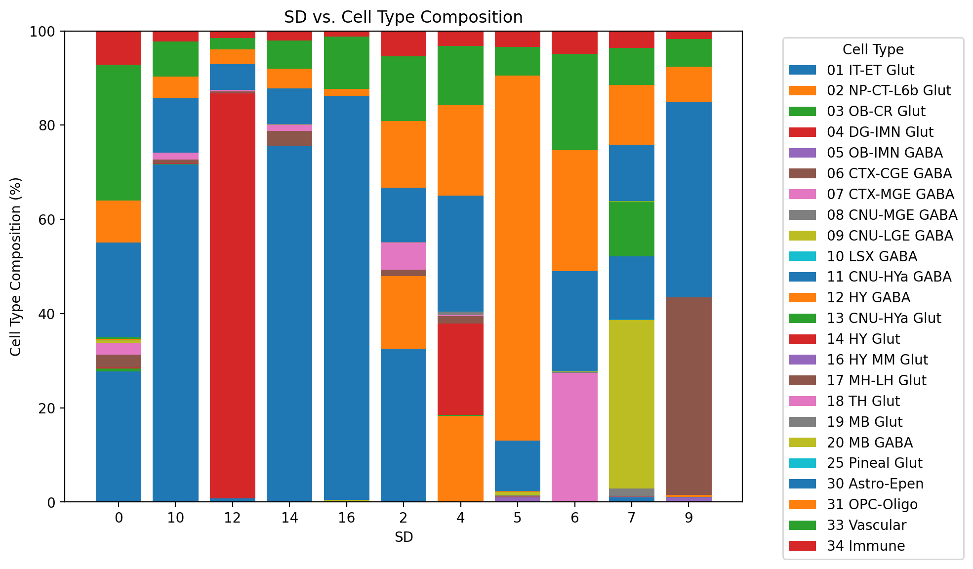
How do the Cell Type compositions of each Spatial Domains change as lambda is increasing?
Additional: access image in the AnnData object
from PIL import Image
import PIL
PIL.Image.MAX_IMAGE_PIXELS = None
adata = sc.datasets.visium_sge(sample_id="V1_Mouse_Brain_Sagittal_Posterior")
adata.var_names_make_unique()
adata.var["mt"] = adata.var_names.str.startswith("MT-")
sc.pp.calculate_qc_metrics(adata, qc_vars=["mt"], inplace=True)sc.pp.filter_cells(adata, min_counts=5000)
sc.pp.filter_cells(adata, max_counts=35000)
adata = adata[adata.obs["pct_counts_mt"] < 20].copy()
print(f"#cells after MT filter: {adata.n_obs}")
sc.pp.filter_genes(adata, min_cells=10)adataprint('Number of spots in the GE matrix (section1, IN TISSUE): ', adata.shape[0])img_path = "10X_Visium_Mouse_Brain_Sagittal_Posterior/spatial/tissue_hires_image.png"
img = Image.open(img_path).convert('RGB')plt.imshow(img)plt.rcParams["figure.figsize"] = (8, 8)
sc.pl.spatial(adata, img_key="hires", color=["total_counts", "n_genes_by_counts"])sc.pp.pca(adata)
sc.pp.neighbors(adata)
sc.tl.umap(adata)
sc.tl.leiden(adata, key_added="clusters", flavor="igraph", directed=False, n_iterations=2)plt.rcParams["figure.figsize"] = (8, 8)
sc.pl.spatial(adata, img_key="hires", color=["clusters"]) # leiden# cluster marker genes
adata.var_names_make_unique()
sc.tl.rank_genes_groups(adata, "clusters", method="t-test")
sc.pl.rank_genes_groups_heatmap(adata, groups="9", n_genes=10, groupby="clusters")sc.pl.spatial(adata, img_key="hires", color=["Ddn"])